3 IGV-Browse
3.1 Overview
3.1.1 Function Overview
JBrowse Eucalyptus Special Edition supports flexible combination of multiple views and tracks, adapting to the full-process research needs of Eucalyptus genomes. It provides a one-stop interactive visualization platform for Eucalyptus functional gene mining, genetic diversity analysis, and molecular breeding.
3.1.2 Supported File Formats
To ensure smooth loading and analysis of Eucalyptus genomic data, the platform supports the following file formats with specific requirements for indexing and version consistency:
Format: FASTA
Requirements: Requires a matching index file (.fai) generated via samtools faidx command. Ensures sequence integrity and efficient loading.
Formats: GFF3, GTF
Requirements: Genome version of the annotation file must be consistent with the reference sequence (e.g., hg38 annotations correspond to hg38 reference sequence).
Formats: VCF, VCF.gz
Requirements: VCF.gz files require a matching tabix index file (.tbi) generated via tabix -p vcf to improve loading efficiency.
Format: BAM
Requirements: Requires a matching index file (.bai) generated via samtools index. Supports filtering by alignment quality thresholds.
Format: BigWig
Features: Compressed format supporting fast loading, ideal for gene expression, methylation, and other quantitative data.
Format: PAF
Generation: Produced by alignment tools such as minimap2, containing Query/Target sequence coordinates and similarity information.
Format: Hi-C (.hic)
Features: Built-in multi-resolution indexes (10kb-1Mb), no additional index upload required.
Format: BED
Usage: Annotates custom genomic intervals (e.g., regulatory regions) in "chromosome + start and end coordinates" format.
3.2 Operation Demonstration
3.2.1 Menu Explanation and Basic Operations
3.2.1.1 FILE Menu
Used for session management and data track import, supporting independent workflows and historical environment recovery.
Creates a brand-new initial session interface with all configurations and content reset to default, for starting independent operation processes.
Imports JSON-format session files saved via "Export Session" to quickly restore historical operating environments and retrieve previous configurations.
Exports current session configurations and content as a JSON file, facilitating backup and migration via subsequent "Import Session".
Copies the current session to generate an identical copy, retaining all configurations and content for independent operations without affecting the original.
Displays a list of recent operation records; clicking list items directly reverts to the corresponding historical session interface.
Provides an entry for adding data tracks (e.g., genomic data tracks) to support data visualization and analysis.

Figure 3.1: Screenshot of FILE Menu in IGV-Browse, showing options for session management and track import
3.2.1.2 ADD Menu
Provides multiple visualization views to adapt to different Eucalyptus genomic analysis scenarios; select the appropriate view based on research objectives.
Displays genomic data in linear form, supporting visualization and analysis of sequences, annotations, and other information for linear genomes.
Presents genomic data in circular form, designed for circular genomes (e.g., Eucalyptus mitochondria) to visualize circular sequence characteristics.
Visualizes sequence alignments via dotplots, intuitively displaying similarities and differences between sequences for homology analysis.
Displays linear synteny relationships between different genomes or chromosomes, aiding in collinearity analysis and homologous region identification.
Presents genome-related data in spreadsheet format, supporting tabular viewing, filtering, and management for efficient data organization.
Detects and analyzes genomic structural variations (SV), parsing breakpoint details and verifying variation authenticity with alignment data.
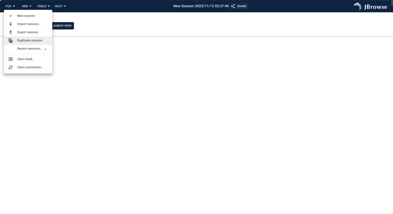
Figure 3.2: Screenshot of ADD Menu in IGV-Browse, showing selectable visualization views for Eucalyptus genomic analysis
3.2.1.3 TOOLS Menu
Integrates utility functions for operation correction, function expansion, and data management, enhancing analysis flexibility and efficiency.
Undo reverses the previous operation to correct errors; Redo reapplies the undone operation to restore the previous state, enhancing operational flexibility.
Provides access to the plugin store for browsing and installing extension plugins, expanding software functions (e.g., custom analysis tools).
Manages genomic assembly data, supporting import, configuration, and deletion of assembly sequences to lay the data foundation for genomic analysis.
Supports theme color switching, with preset light/dark themes or custom color schemes to adapt to different visual habits and usage scenarios.
Displays and manages running tasks, allowing users to view task progress and status for better process control.
Saves important genomic regions as bookmarks for quick access to target regions, improving analysis efficiency.
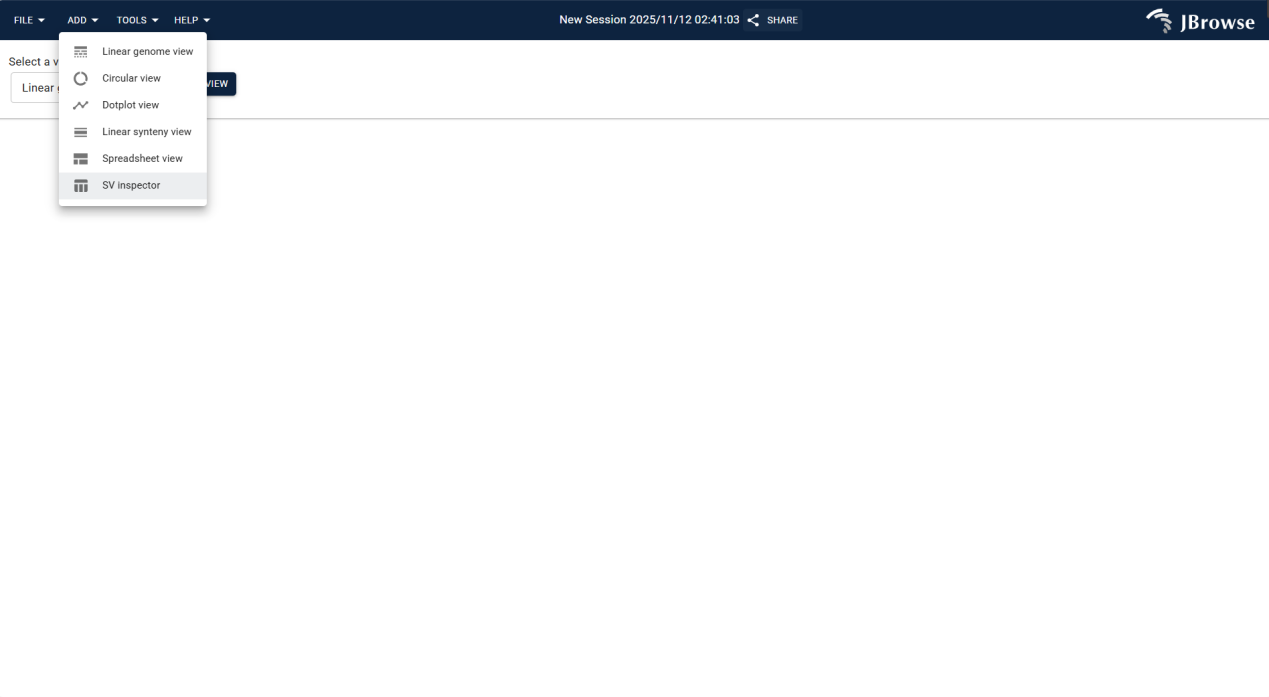
Figure 3.3: Screenshot of TOOLS Menu in IGV-Browse, showing utility functions for operation management and function expansion
3.2.2 Independent File Import
Upload Eucalyptus reference genome files (FASTA format) and matching index files via Assembly Manager; follow the steps below:
Click TOOLS in the top menu bar and select Assembly Manager from the drop-down menu. This is the core entry for managing all genomic assemblies.
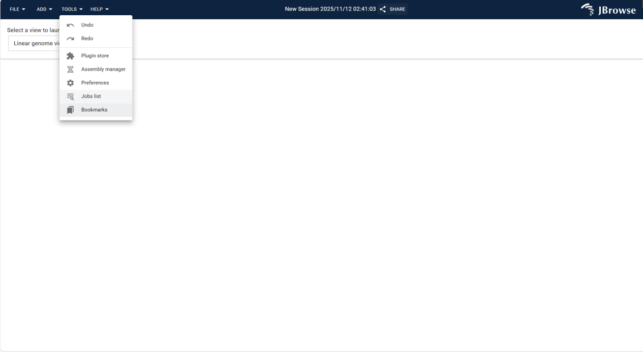
Figure 3.4: Screenshot of accessing Assembly Manager via TOOLS Menu in IGV-Browse
After opening Assembly Manager, view the list of existing genomic assemblies. Click the ADD NEW ASSEMBLY button at the bottom to pop up the configuration window.
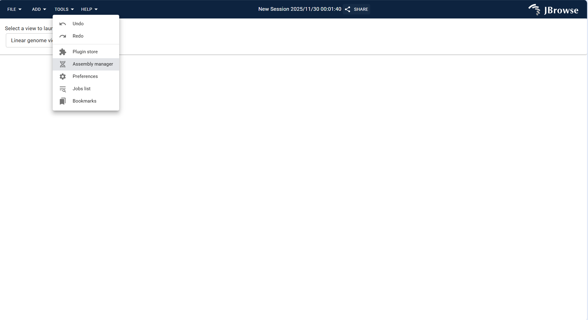
Figure 3.5: Screenshot of accessing Assembly Manager via TOOLS Menu in IGV-Browse
- Assembly Name: Enter the assembly identifier (e.g.,
Eucalyptus_grandis_v2.0.fa), consistent with the logical file name. - Assembly Display Name (optional): Enter a readable name (e.g.,
Eucalyptus grandis (v2.0)) to distinguish assemblies. - Adapter Type: Select IndexedFastaAdapter (default for FASTA-format genomes).
- fastaLocation: Upload the FASTA-format genome file via local file or online URL.
- faiLocation: Upload the matching .fai index file (generated via
samtools faidxcommand).
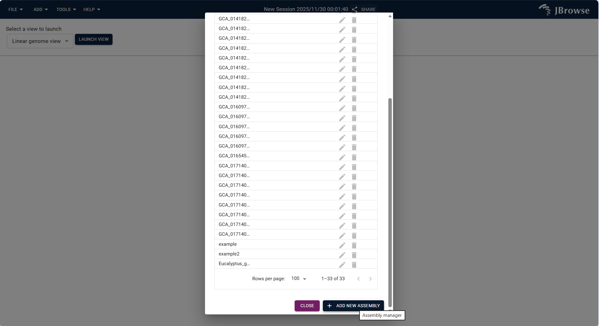
Figure 3.6: Screenshot of accessing Assembly Manager via TOOLS Menu in IGV-Browse
Click SUBMIT to verify file integrity. If successful, the new assembly is added to the list, and a "Added [Assembly Name]" prompt pops up.
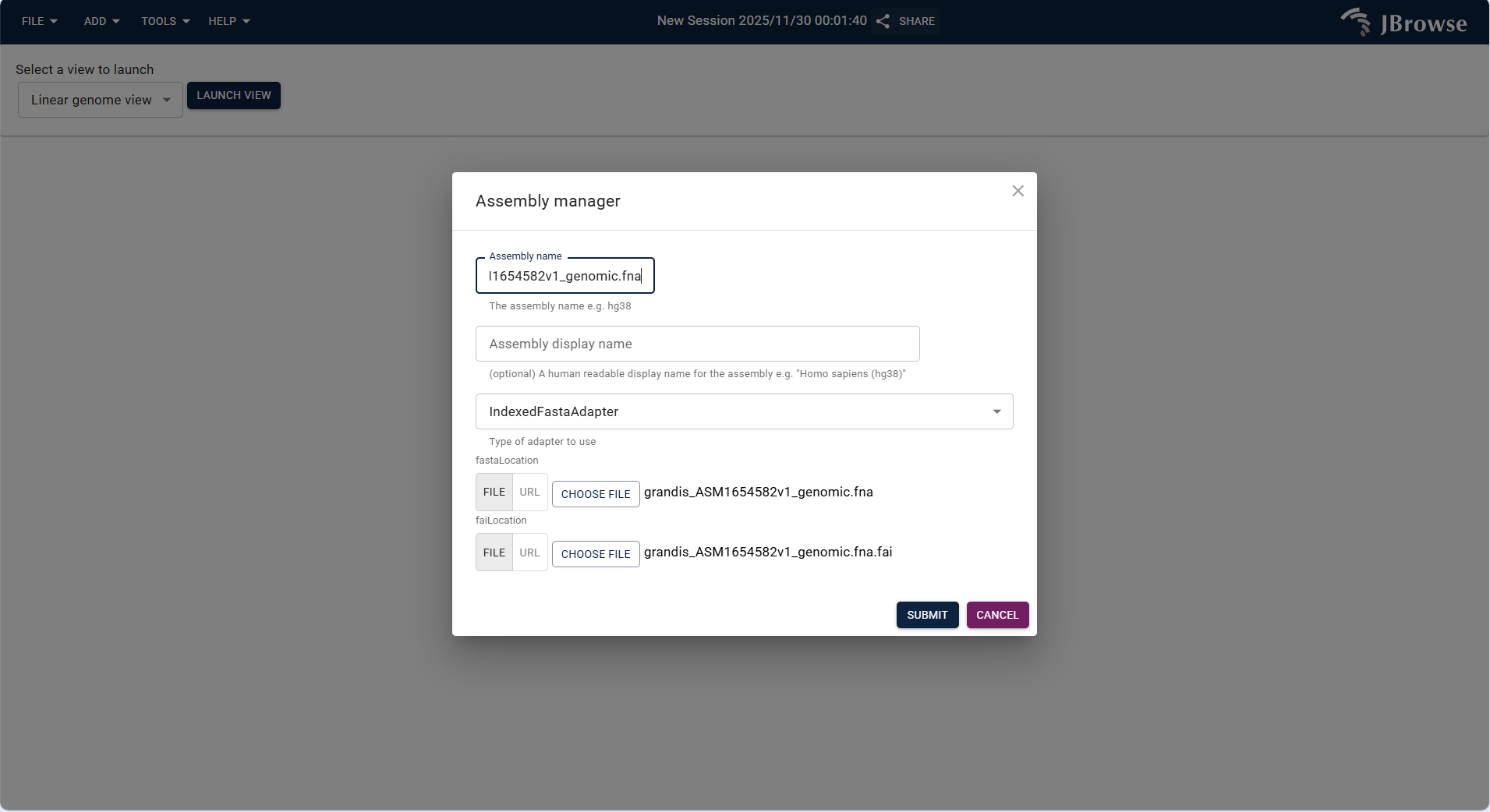
Figure 3.7: Screenshot of accessing Assembly Manager via TOOLS Menu in IGV-Browse
3.2.3 Core Track Operations (Visualization + Track Manipulation)
This section details the operation steps for different track types under various views, including track addition, parameter configuration, and result visualization. All operations are based on Eucalyptus genomic data analysis scenarios, ensuring practicality and operability.
3.2.3.1 Linear Genome View + Different Type Tracks
Linear Genome View is the most commonly used view in Eucalyptus genome analysis, supporting the superposition of multiple track types to realize comprehensive analysis of target regions. The operation steps for each track type are as follows:
(1) Linear Genome View + Reference Sequence Track*
- Select a target genome from the JBrowse genome list (e.g.,
grandis_ASM1654582v1_genomic.fnahuman genome) or upload your own FASTA-format genome/protein file. - After selecting the genome, enter or select the target chromosome (e.g., NC_052612.1) and click "OPEN" to enter the view.
- Click "OPEN TRACK SELECTOR" to open the track selection panel, find and check "Reference sequence (grandis_ASM1654582v1_genomic.fna)" to load the reference sequence track.
- Due to the large span of the genome sequence, use the zoom tool or select a chromosome interval (e.g., NC_052612.1:92,780,830..92,780,854) to zoom in, and you can clearly view the base sequence and corresponding amino acid information.
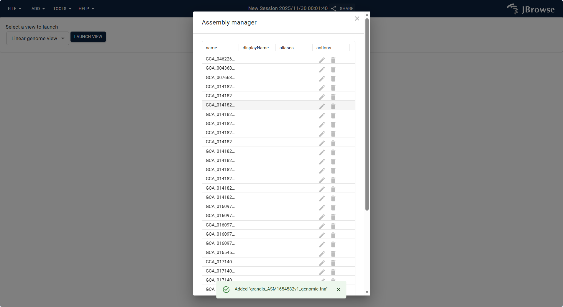
Figure 3.8: Screenshot of Linear Genome View with overlaid Reference track
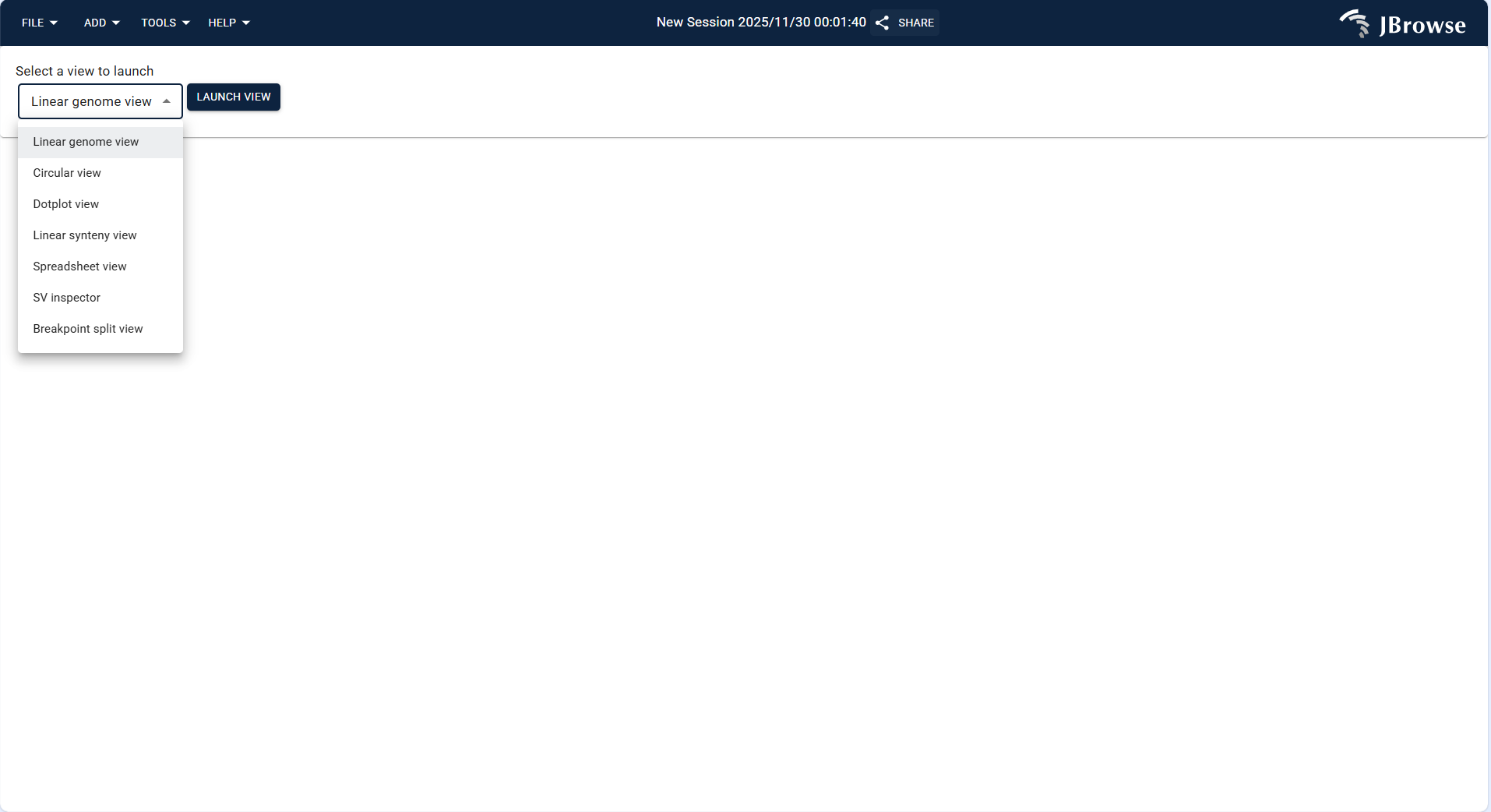
Figure 3.9: Screenshot of Linear Genome View with overlaid Reference track
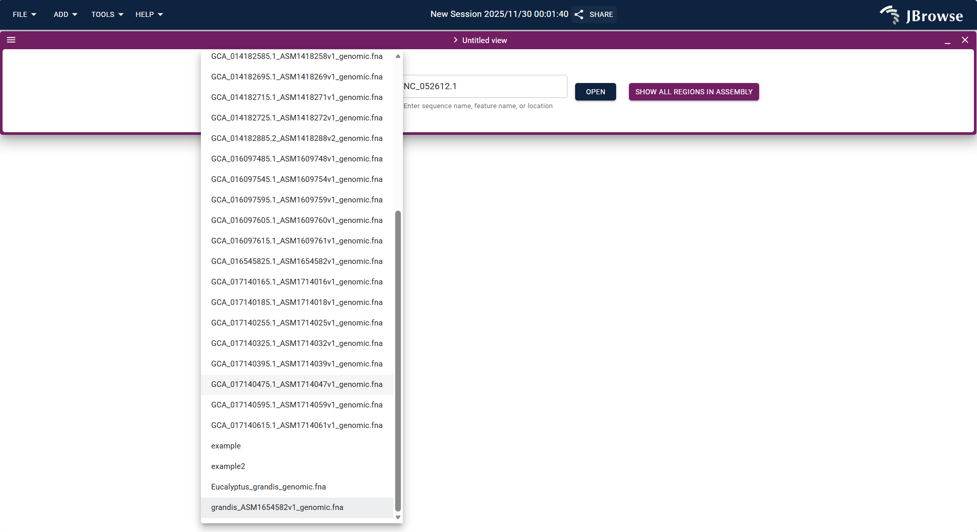
Figure 3.10: Screenshot of Linear Genome View with overlaid Reference track
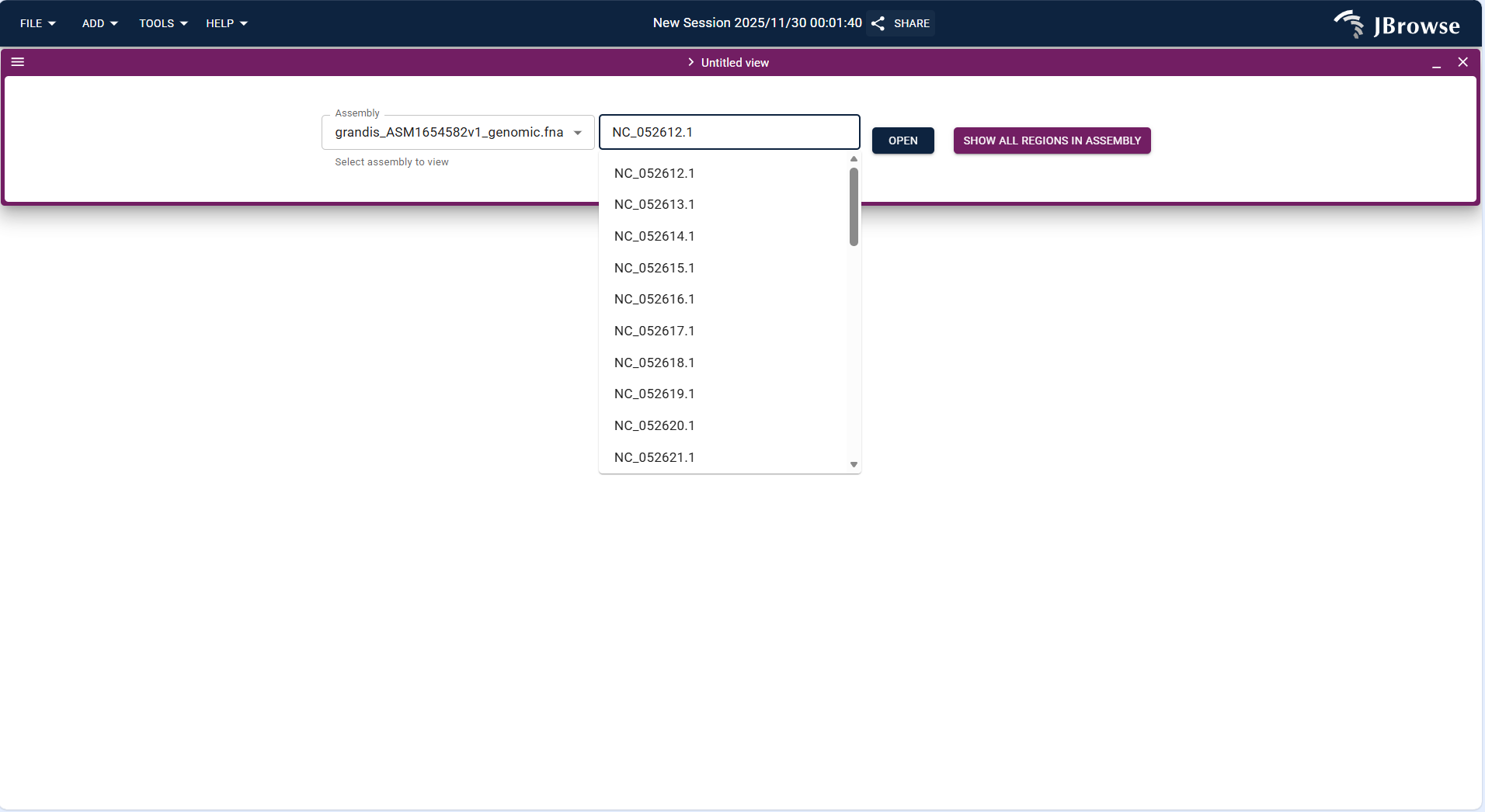
Figure 3.11: Screenshot of Linear Genome View with overlaid Reference track
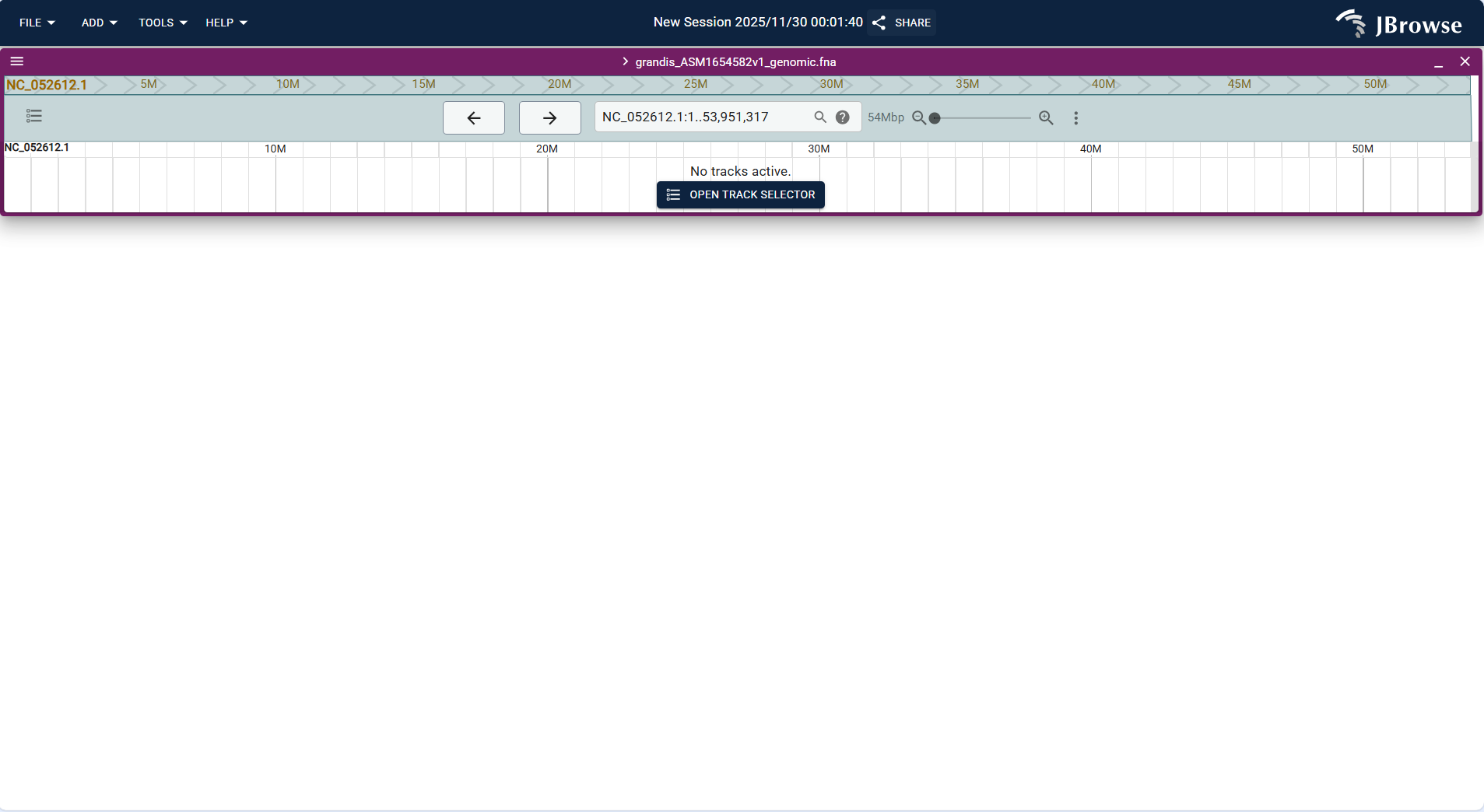
Figure 3.12: Screenshot of Linear Genome View with overlaid Reference track
- Click the top menu bar FILE → Open track... to start the track addition workflow.
- In the "Enter track data" step, select a local file or enter a URL to upload an annotation file (supports GFF3, GTF formats; example:
grandis_ASM1654582v1_genomic.gff). - In the "Confirm track type" step, the system automatically identifies the track type as "Feature track", confirm the assembly is the target genome (e.g., grandis_ASM1654582v1_genomic.fna), and click "ADD" to complete the addition.
- After loading, the Feature track is overlaid with the Reference sequence track, allowing intuitive viewing of the association between gene annotations (e.g., gene structure, transcripts) and the reference sequence.
- Basic Track is used to display custom genomic interval information (e.g., regulatory regions, repetitive sequence regions) in BED format.
- Operation steps: Click FILE → Open track..., select "BED" as the file type in the "Enter track data" step, upload the BED file (e.g.,
ssr_grandis_NC014570.bed), and confirm the track type as "Basic Track" to complete the addition. - After loading, the track displays the custom interval as a highlighted block, which can be overlaid with other tracks to analyze the correlation between functional regions and genes/variations.
- Alignments Track is used to display sequencing reads alignment data in BAM format, supporting the verification of variation authenticity and alignment quality evaluation.
- Operation steps: Click FILE → Open track..., upload the BAM file (e.g.,
grandis_leaf_align.bam) and its matching index file (.bai) in the "Enter track data" step. The system automatically identifies the track type as "Alignments Track", confirm the assembly, and click "ADD". - After loading, you can adjust the alignment quality threshold to filter low-quality reads, and view the distribution of reads in the target region to assist in variation calling and validation.
- Variant Track is used to display SNP, Indel, and other variation data in VCF/VCF.gz format.
- Operation steps: Click FILE → Open track..., upload the variation data file (example:
grandis_chrom1.vcf) in the "Enter track data" step. The system identifies the track type as "Variant track", confirm the assembly, and click "ADD". - After loading, the track displays variation sites in the target region, which can be overlaid with Feature track to analyze the association between variations and gene structures (e.g., whether variations are located in exons, introns).
- Quantitative Track is used to display continuous quantitative data such as gene expression levels and methylation levels in BigWig format.
- Operation steps: Click FILE → Open track..., upload the BigWig file (example:
grandis_leaf_align.bw) in the "Enter track data" step. The system identifies the track type as "Quantitative track", confirm the assembly, and click "ADD". - After loading, the track displays the data distribution trend as a histogram or curve, which can be combined with Variant track and Feature track to analyze the correlation between gene expression, variation sites, and functional regions.
- Multi-quantitative Track supports simultaneous loading of multiple BigWig files (e.g., expression data of the same gene under different tissues/stress conditions) for comparative analysis.
- Operation steps: Repeat the "Quantitative Track" addition process to upload multiple BigWig files. The system displays each file as an independent sub-track, and you can adjust the color and height of each sub-track for differentiation.
- Application scenario: Compare the expression patterns of Eucalyptus target genes in roots, stems, leaves, and other tissues, or analyze the dynamic changes of gene expression under different stress durations (0h, 6h, 12h, 24h).
- GC Content Track is used to display the GC content distribution in the genome, which is helpful for identifying functional regions (e.g., gene-rich regions often have high GC content).
- Operation steps: Click FILE → Open track..., Select GC content-compatible format files as track data Or select "GC Content" as the track type, set the window size (default 100bp), and the system automatically calculates and generates the GC content track based on the reference genome.
- After loading, the track displays the GC content value of each window as a curve, which can be combined with Feature track to analyze the correlation between GC content and gene distribution.
- Synteny Track is used to display the collinearity relationship between Eucalyptus and related species (e.g., other Myrtaceae plants) in PAF format.
- Operation steps: First generate the PAF file using alignment tools such as minimap2 (e.g., compare grandis_ASM1654582v1_genomic.fna with globulus_ASM4622685v1_genomic.fna), then click FILE → Open track... to upload the PAF file. The system identifies the track type as "SyntenyTrack", set the query and target assemblies, and click "ADD".
- After loading, the track marks homologous segments with connecting lines, which can be used to analyze genome evolution events such as chromosome rearrangement and inversion.
- Hi-C Track is used to display chromatin interaction data in dedicated .hic format, supporting the analysis of three-dimensional genome structures such as topological associated domains (TADs).
- Operation steps: Click FILE → Open track..., upload the .hic file (example:
GSE63525_GM12878_diploid_maternal.hic) in the "Enter track data" step. The system identifies the track type as "Hi-C track", confirm the assembly, and click "ADD". - After loading, the track displays interaction intensity as a heatmap (darker colors indicate stronger interactions), which can be combined with other tracks to analyze the correlation between three-dimensional genome structure, gene expression, and variation sites.
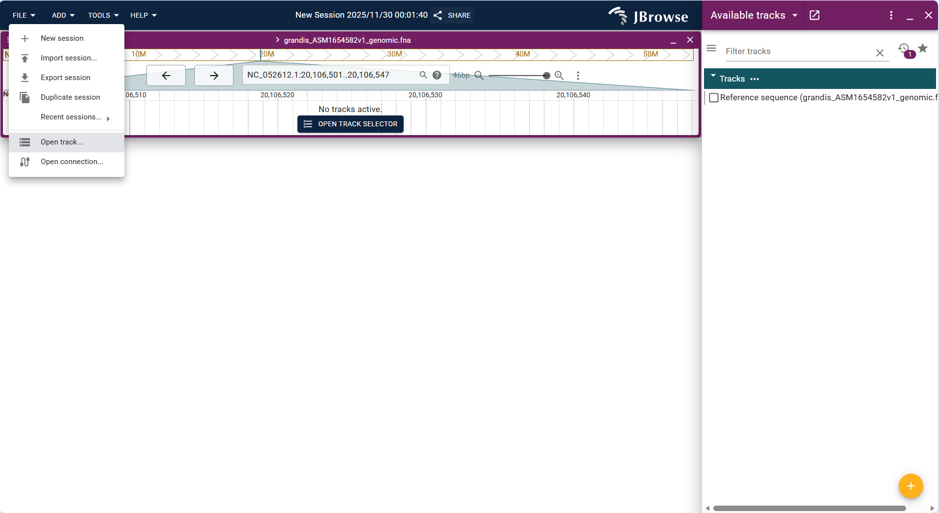
Figure 3.13: Screenshot of Linear Genome View with overlaid Feature, Variant,Quantitative tracks and so on.
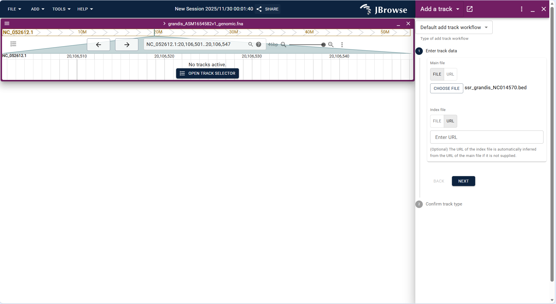
Figure 3.14: Screenshot of Linear Genome View with overlaid Feature, Variant,Quantitative tracks and so on.
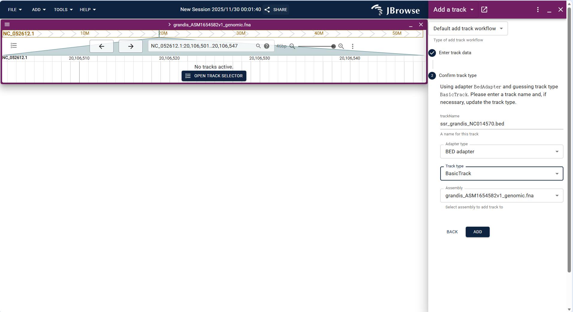
Figure 3.15: Screenshot of Linear Genome View with overlaid Feature, Variant,Quantitative tracks and so on.
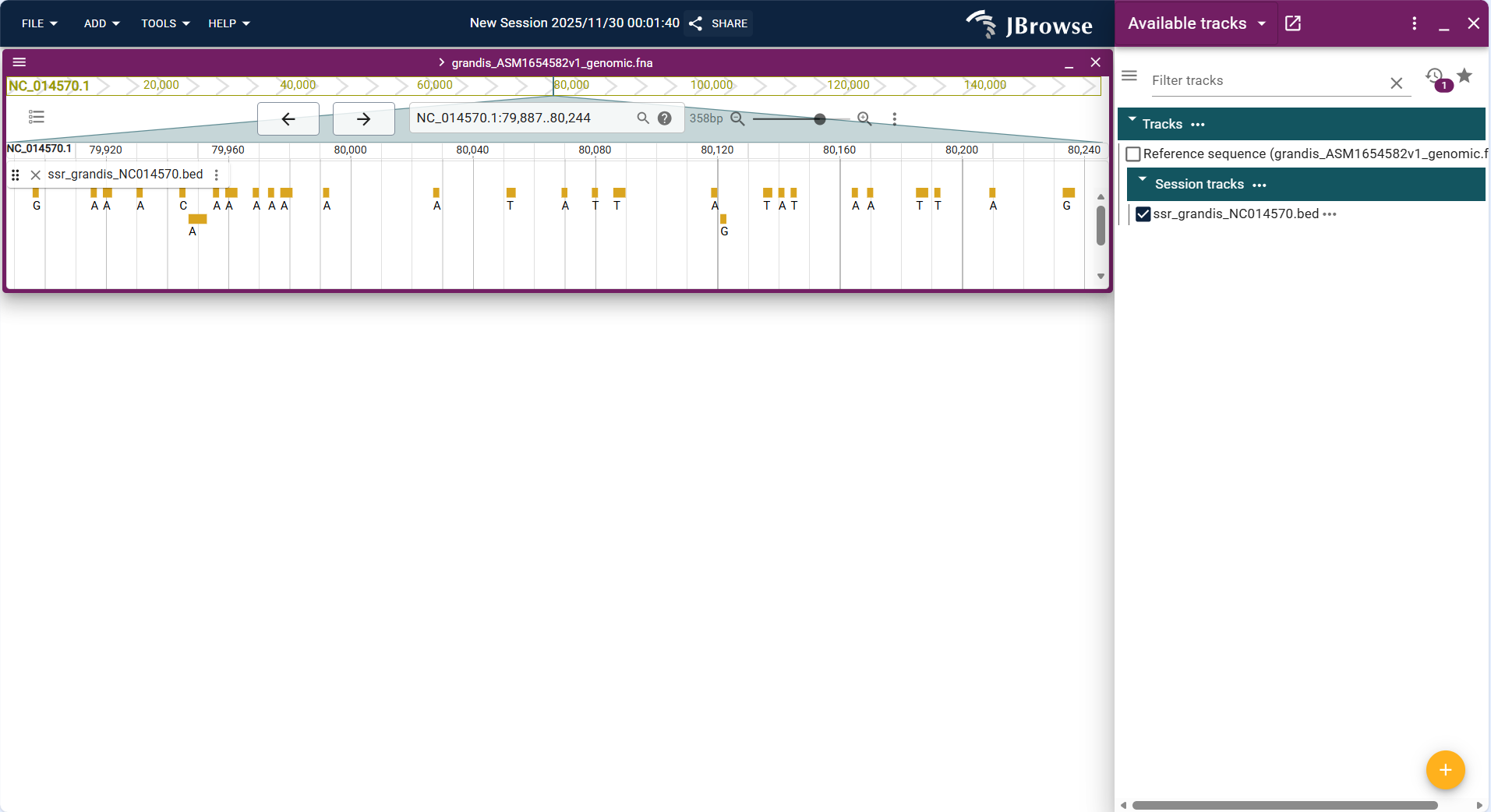
Figure 3.16: Screenshot of Linear Genome View with overlaid Feature, Variant,Quantitative tracks and so on.
3.2.3.2 Circular View + Different Type Tracks
Circular View is suitable for circular genomes such as Eucalyptus mitochondria and chloroplasts, supporting the display of reference sequences, annotations, and other tracks in a circular layout. The operation steps for each track type are as follows:
- Upload the VCF/VCF.gz format variation file of the circular genome (e.g.,
Eucalyptus_mitochondria_variants.vcf.gz) and its index file via FILE → Open track.... - The system identifies the track type as "Variant track", confirm the assembly, and click "ADD" to load the track.
- After loading, variation sites are marked on the circular genome, which can be combined with Feature track to analyze whether variations are located in functional regions (e.g., coding regions of key genes).

Figure 3.17: Screenshot of Circular View showing Eucalyptus genome with multiple tracks
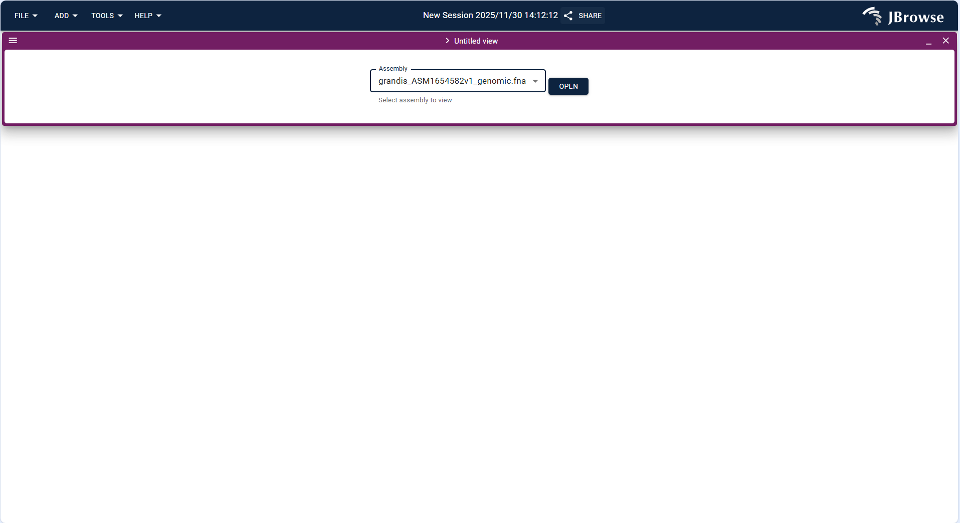
Figure 3.18: Screenshot of Circular View showing Eucalyptus genome with multiple tracks
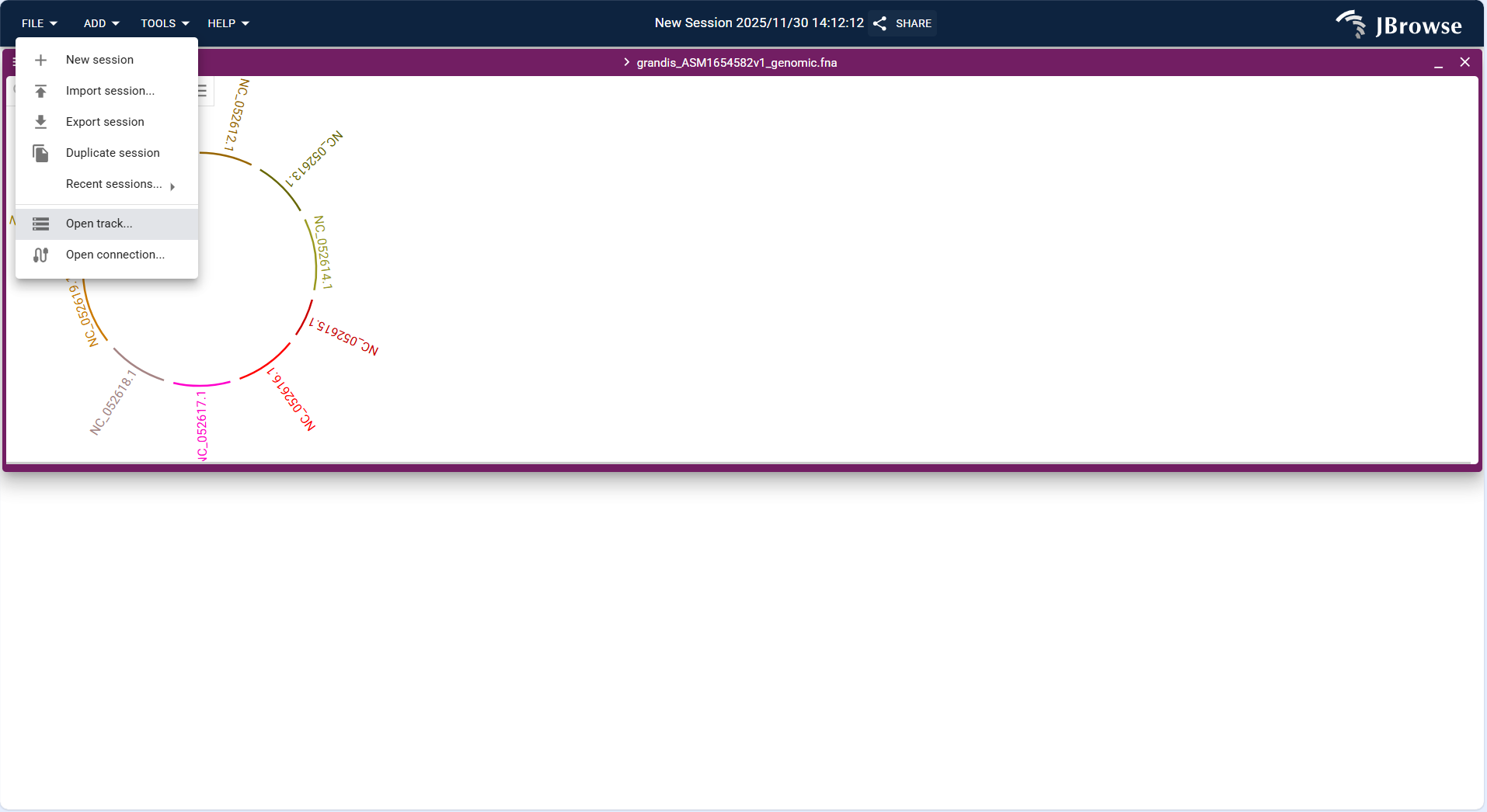
Figure 3.19: Screenshot of Circular View showing Eucalyptus genome with multiple tracks
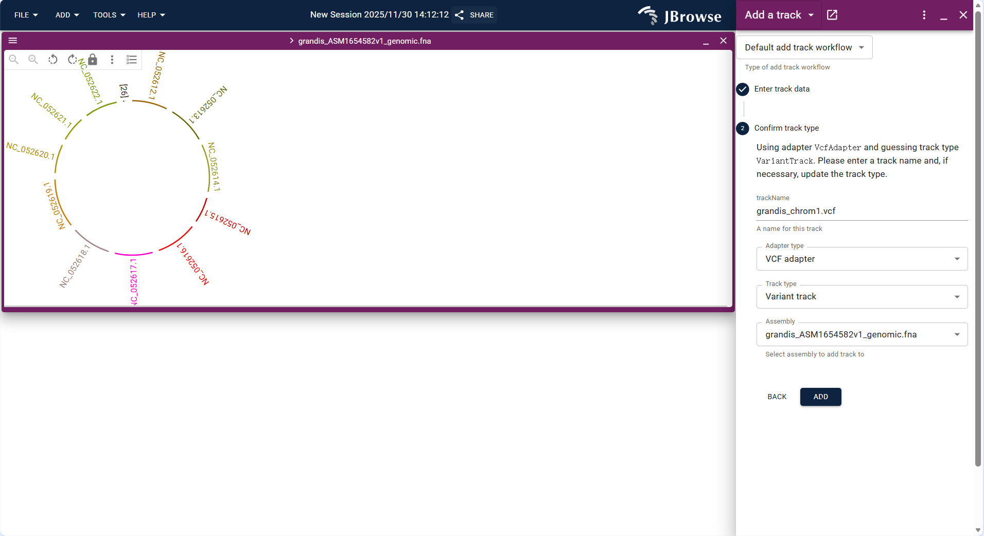
Figure 3.20: Screenshot of Circular View showing Eucalyptus genome with multiple tracks
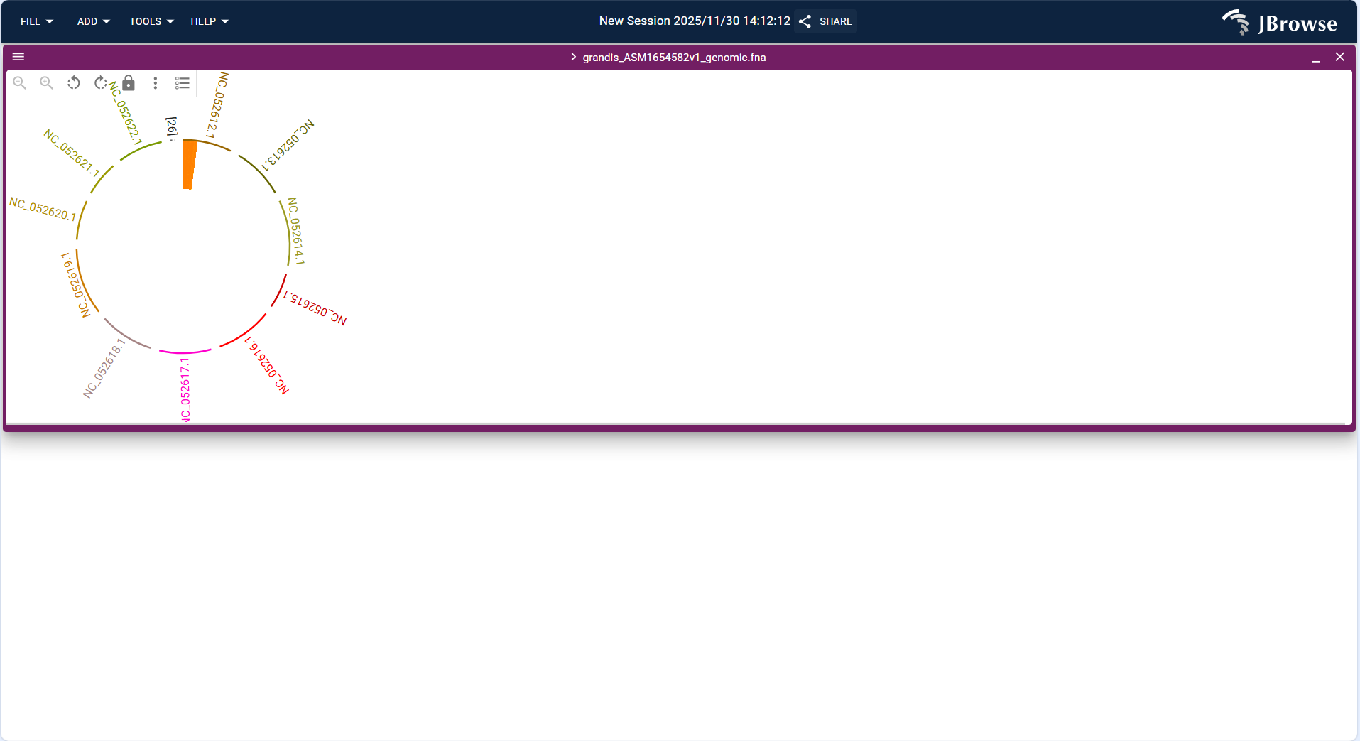
Figure 3.21: Screenshot of Circular View showing Eucalyptus genome with multiple tracks
3.2.3.3 Dotplot View + Track
Dotplot View is mainly used for sequence alignment visualization, supporting the display of collinearity and differences between Eucalyptus and related species' genomes. Currently, it only supports SyntenyTrack loading:
- Click the top menu bar ADD → Dotplot view to create a new dotplot view interface.
- Upload the PAF format collinearity file (e.g.,
e_grandis_globulus_final.paf) via FILE → Open track..., and the system automatically identifies the track type as "SyntenyTrack". - Set the x-axis (query genome, e.g., grandis_ASM1654582v1_genomic.fna) and y-axis (target genome, e.g., globulus_ASM4622685v1_genomic.fna) assemblies, and click "ADD" to load the track.
- After loading, the dotplot uses dots to represent homologous segments (the closer the dots are to the diagonal, the better the collinearity), which can be used to identify chromosome rearrangement events such as inversion and translocation.
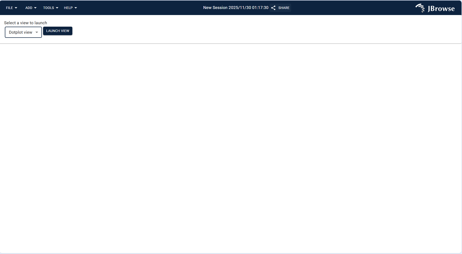
Figure 3.22: Screenshot of Dotplot View with SyntenyTrack, showing collinearity between two genomes
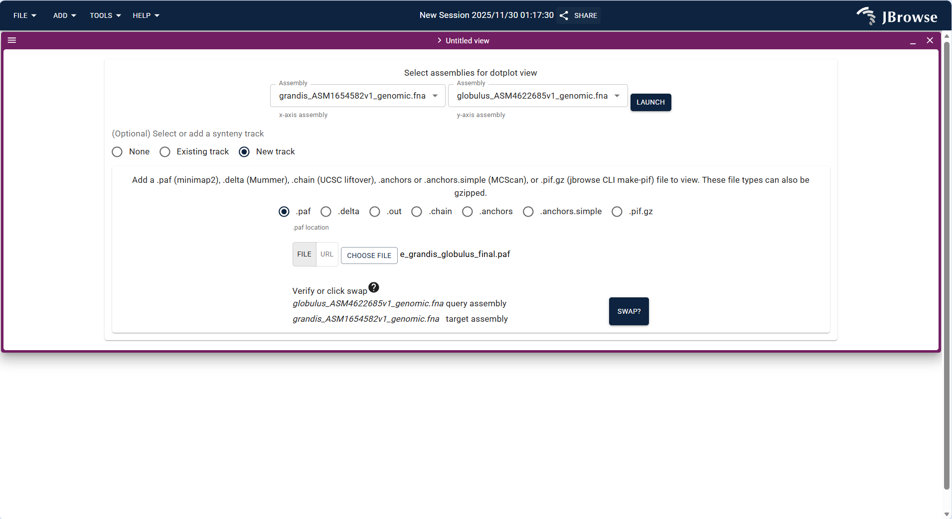
Figure 3.23: Screenshot of Dotplot View with SyntenyTrack, showing collinearity between two genomes
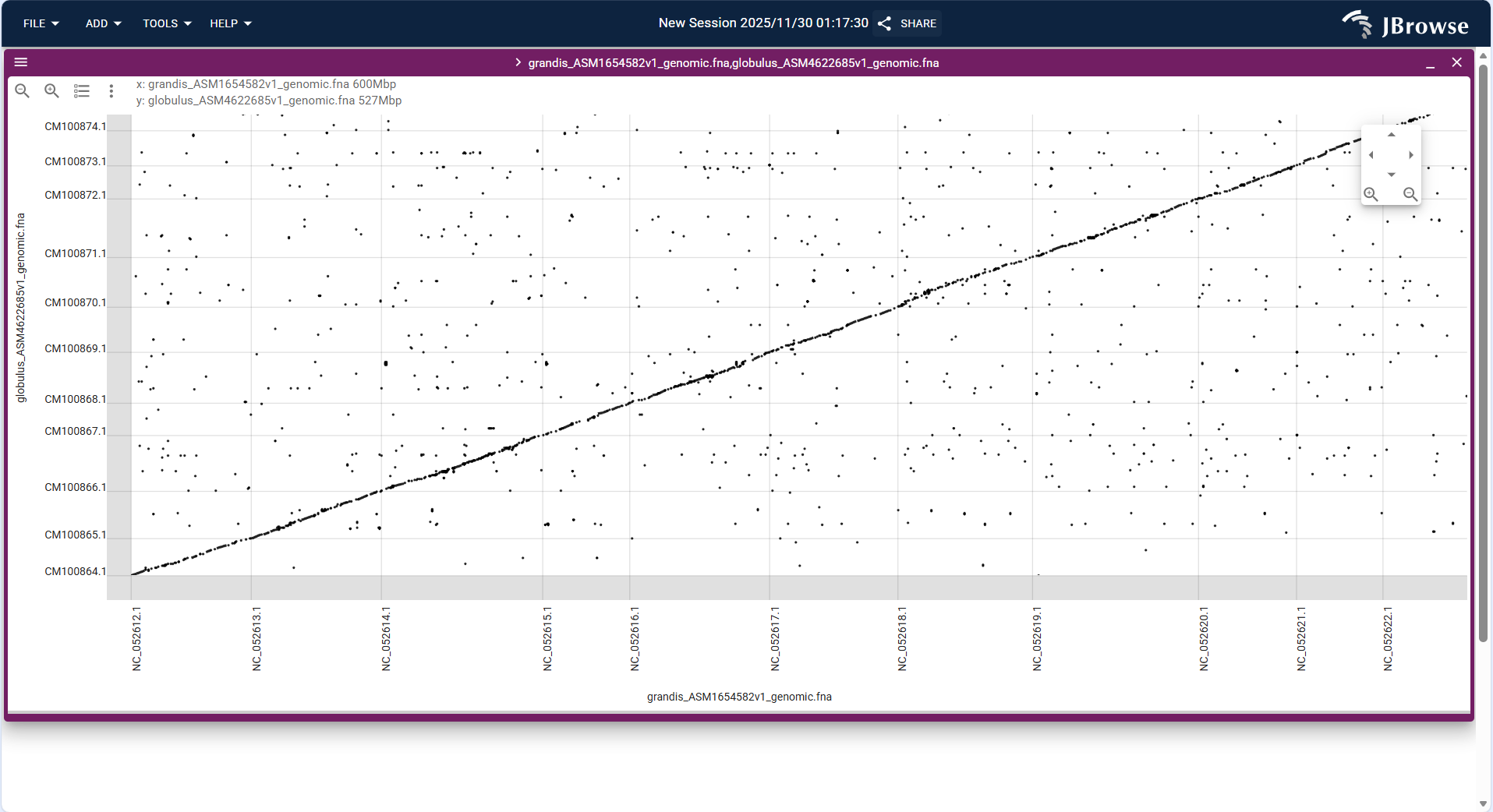
Figure 3.24: Screenshot of Dotplot View with SyntenyTrack, showing collinearity between two genomes
3.2.3.4 Linear Synteny View + Track
Linear Synteny View displays collinearity relationships in a linear layout, which is more intuitive for comparing gene order between Eucalyptus and related species. It only supports SyntenyTrack loading:
- Click the top menu bar ADD → Linear synteny view to create a new linear synteny view interface.
- Upload the PAF format collinearity file (same as Dotplot View) via FILE → Open track..., and set the query and target assemblies.
- After loading, the view displays the chromosomes of the two species in parallel, and uses connecting lines to mark homologous segments, which can clearly show the order of homologous genes and structural variations such as chromosome breaks.
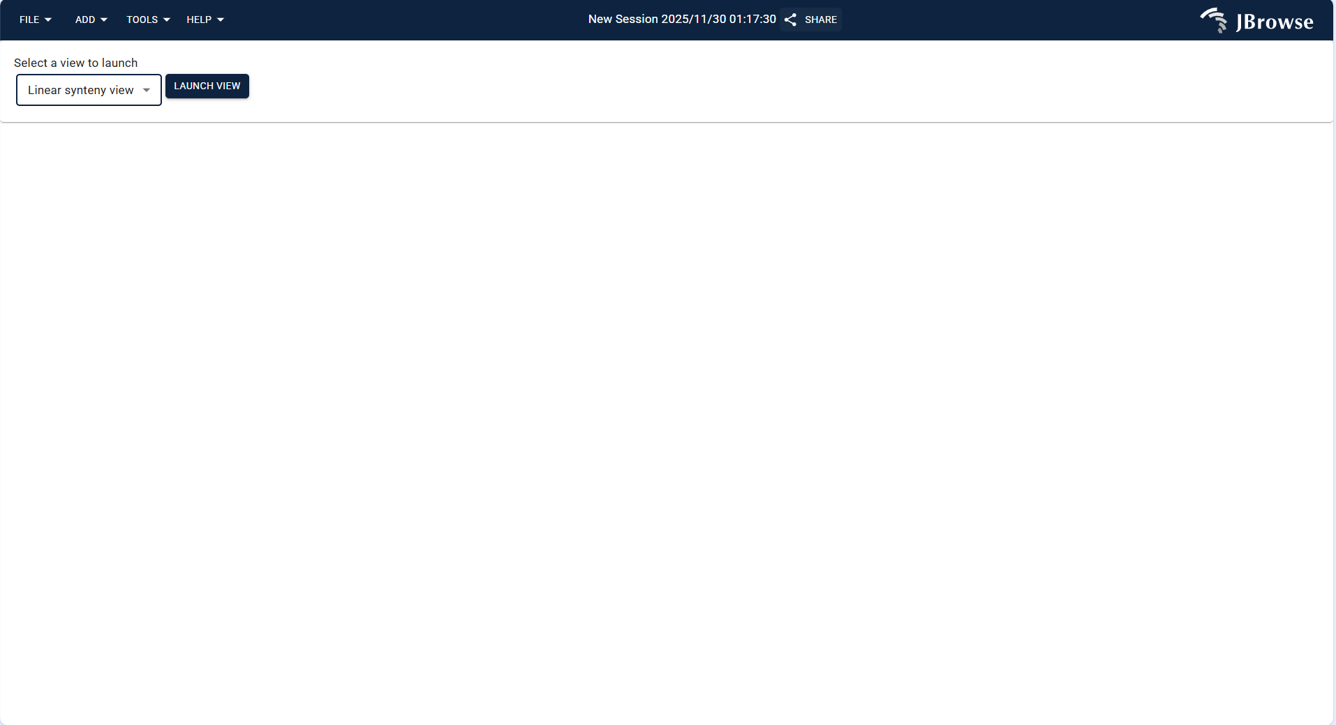
Figure 3.25: Screenshot of Linear Synteny View showing collinearity between Eucalyptus and related species chromosomes
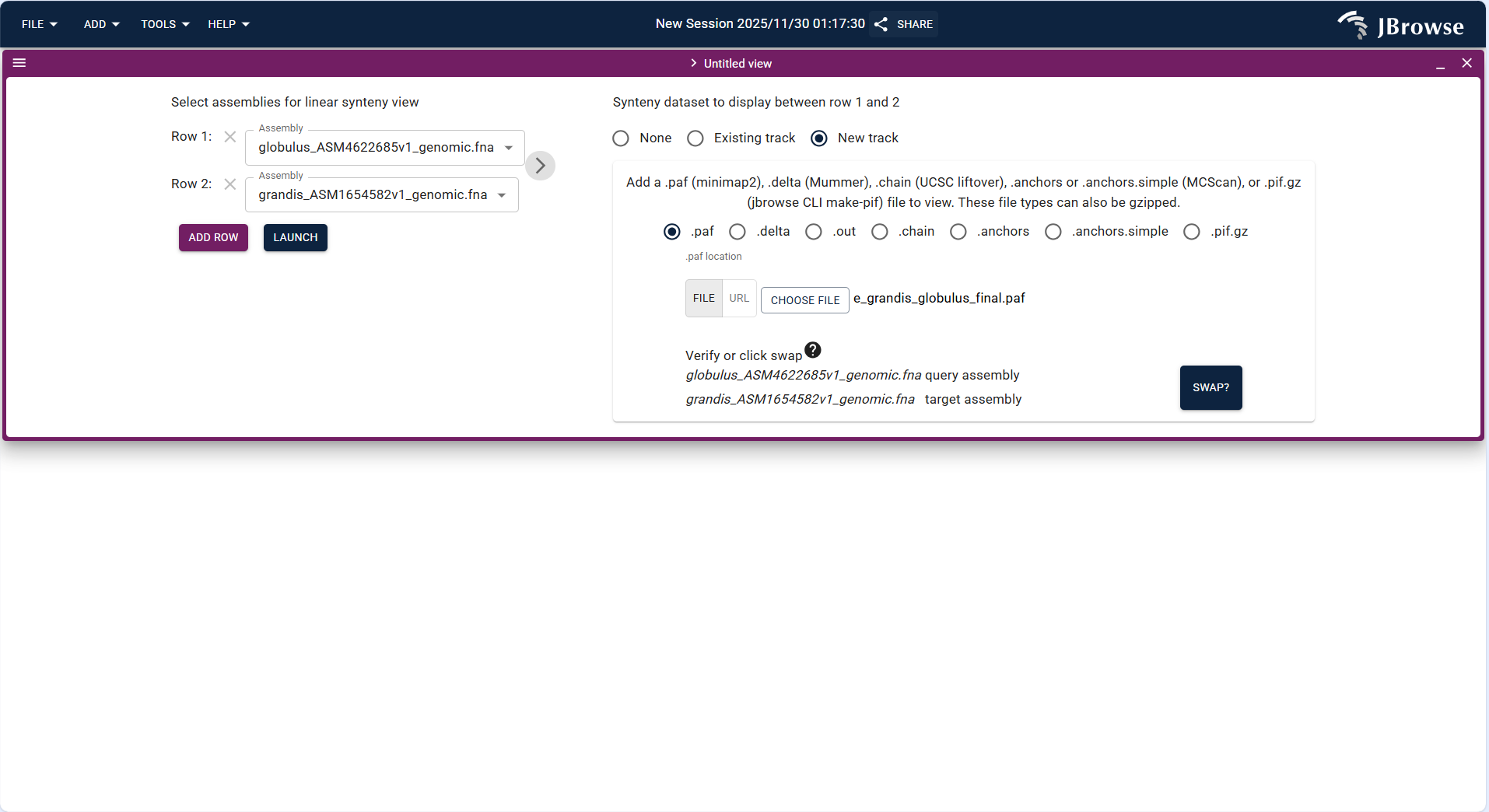
Figure 3.26: Screenshot of Linear Synteny View showing collinearity between Eucalyptus and related species chromosomes
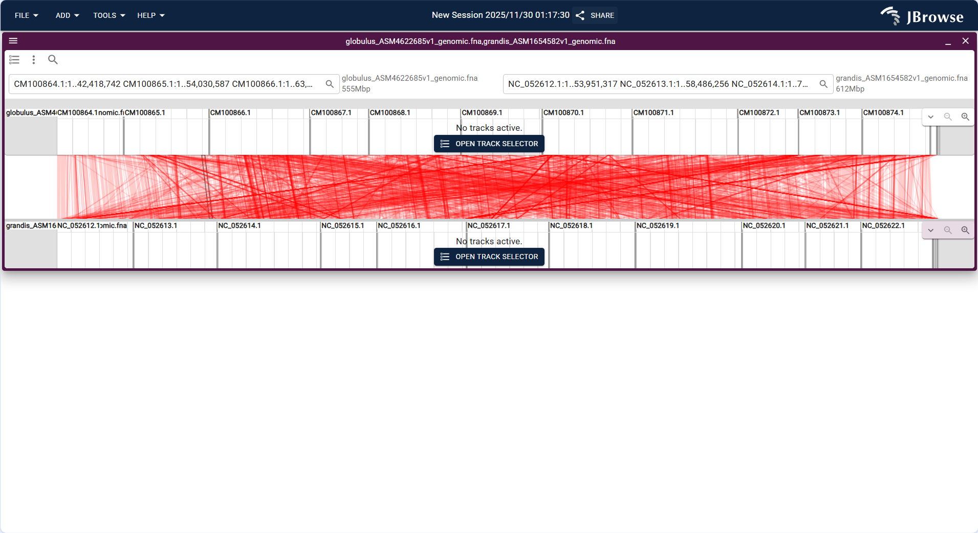
Figure 3.27: Screenshot of Linear Synteny View showing collinearity between Eucalyptus and related species chromosomes
3.2.3.5 Spreadsheet View + Different Type Tracks
Spreadsheet View displays genomic data in a table format, supporting batch filtering and management of gene annotations and variation data. It supports Feature track and Variant track loading:
- Click the top menu bar ADD → Spreadsheet view to create a new spreadsheet view interface.
- Upload the GFF3/GTF format annotation file via FILE → Open track..., and the system identifies the track type as "Feature track".
- After loading, the table displays gene-related information (e.g., Gene ID, chromosome location, functional annotation) in rows and columns, supporting batch filtering by conditions (e.g., screening genes located on NC_052612.1).
- Upload the VCF/VCF.gz format variation file and its index file via FILE → Open track..., and the system identifies the track type as "Variant track".
- After loading, the table displays variation-related information (e.g., variation position, reference allele, alternative allele, quality value) in rows and columns, supporting batch filtering of high-quality variations (e.g., QUAL > 30).
- Supports CSV format export of filtered data for further statistical analysis in software such as Excel or R.
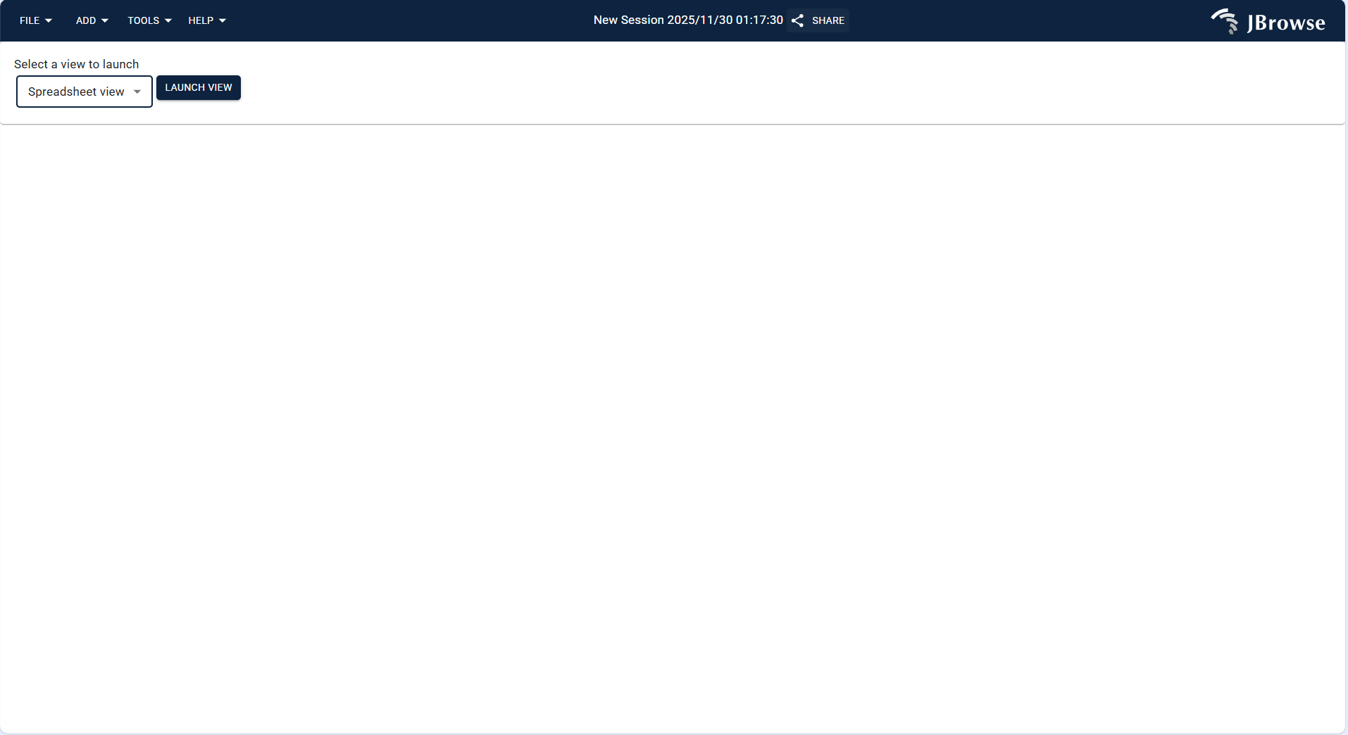
Figure 3.28: Screenshot of Spreadsheet View displaying feature and variation data in table format
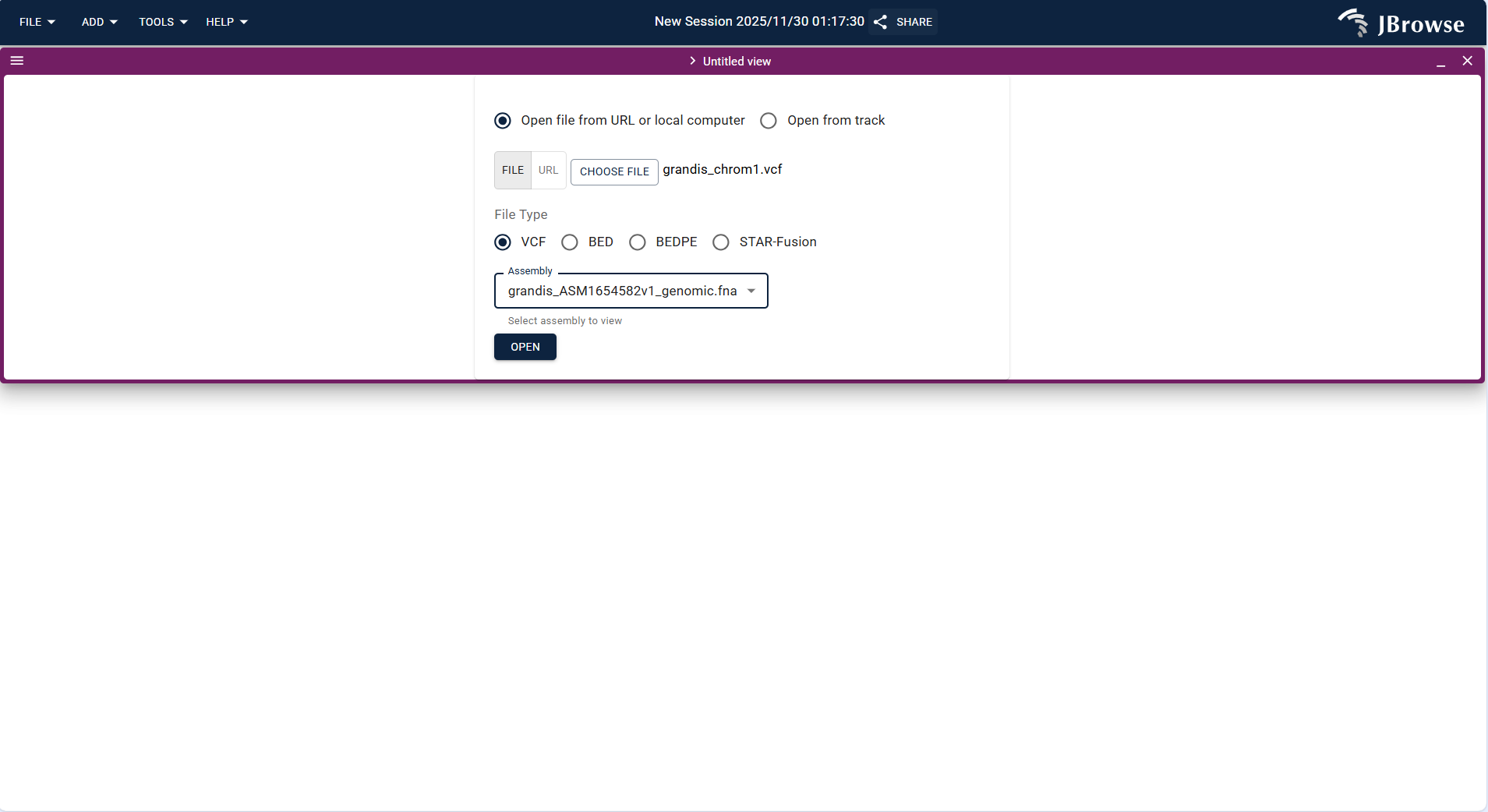
Figure 3.29: Screenshot of Spreadsheet View displaying feature and variation data in table format
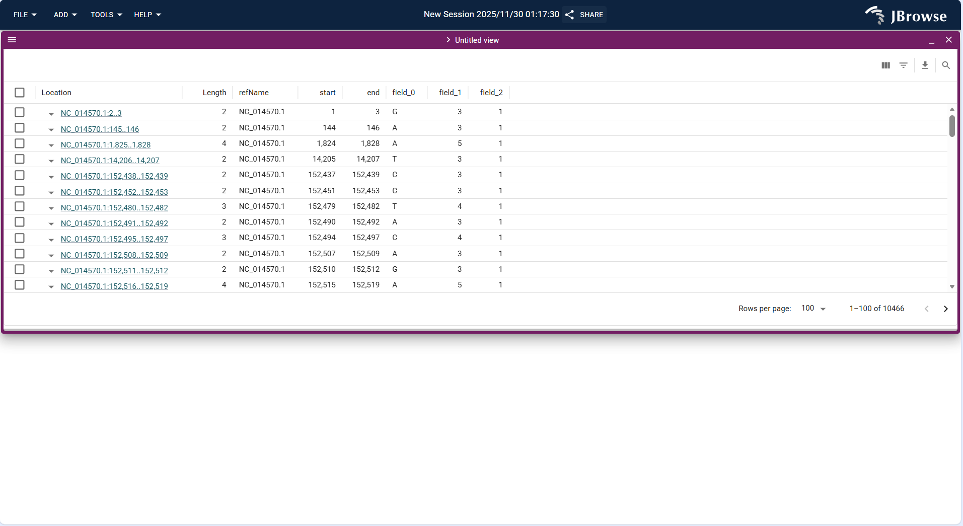
Figure 3.30: Screenshot of Spreadsheet View displaying feature and variation data in table format
3.2.3.6 SV Inspector + Track
SV Inspector is a dedicated tool for structural variation analysis, supporting detailed parsing of Eucalyptus genome structural variations (e.g., deletions, duplications) and only supports Variant track loading:
- Click the top menu bar ADD → SV inspector to create a new SV Inspector interface.
- Upload the VCF/VCF.gz format structural variation file (containing SV annotations such as DEL, DUP) and its index file via FILE → Open track....
- The system loads the Variant track and displays structural variation breakpoints in a dedicated window, supporting zooming in to view breakpoint details and alignment data verification (combined with Alignments Track).
- Application scenario: Verify the authenticity of predicted structural variations in Eucalyptus genome and analyze the impact of structural variations on gene structure (e.g., whether deletions lead to gene fragment loss).
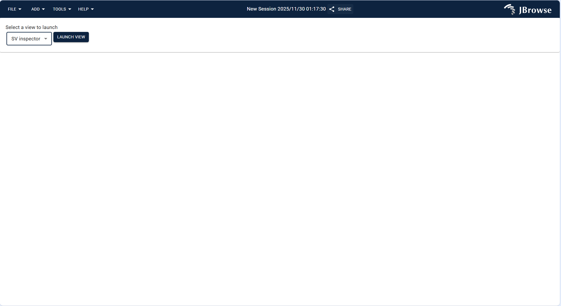
Figure 3.31: Screenshot of SV Inspector verifying Eucalyptus genome structural variation
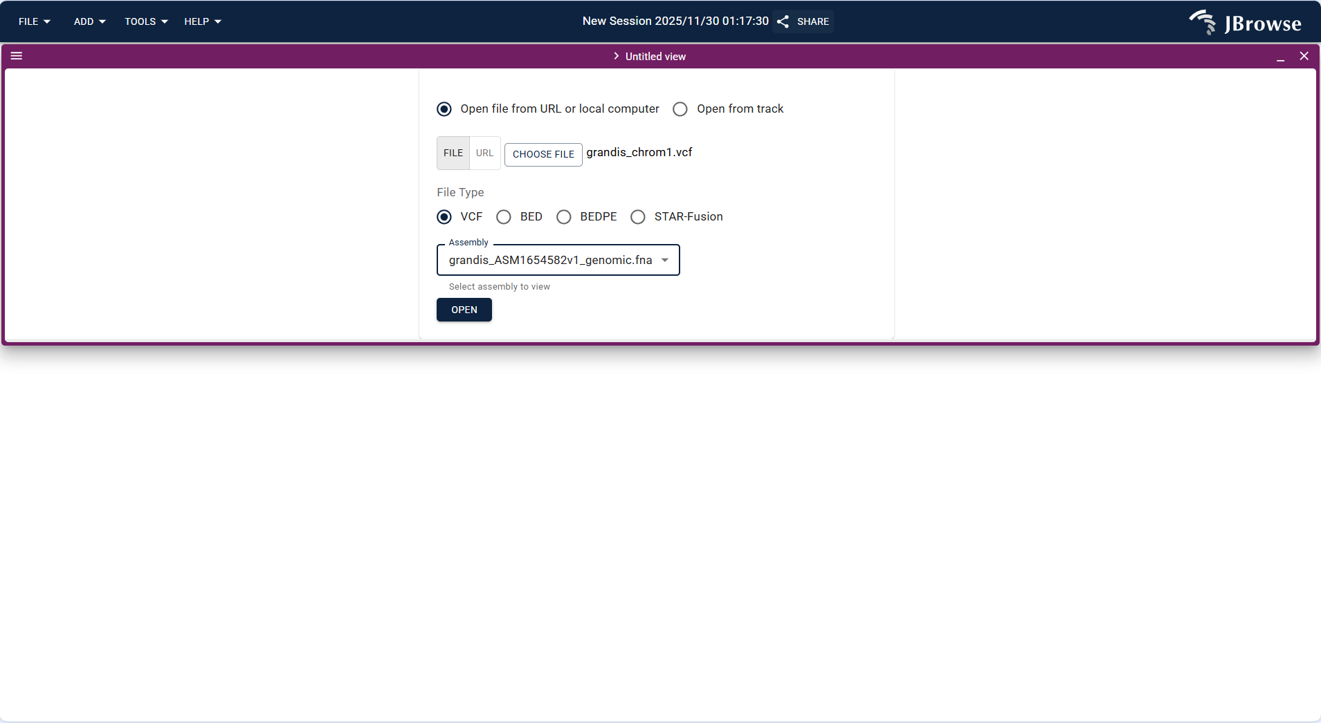
Figure 3.32: Screenshot of SV Inspector verifying Eucalyptus genome structural variation
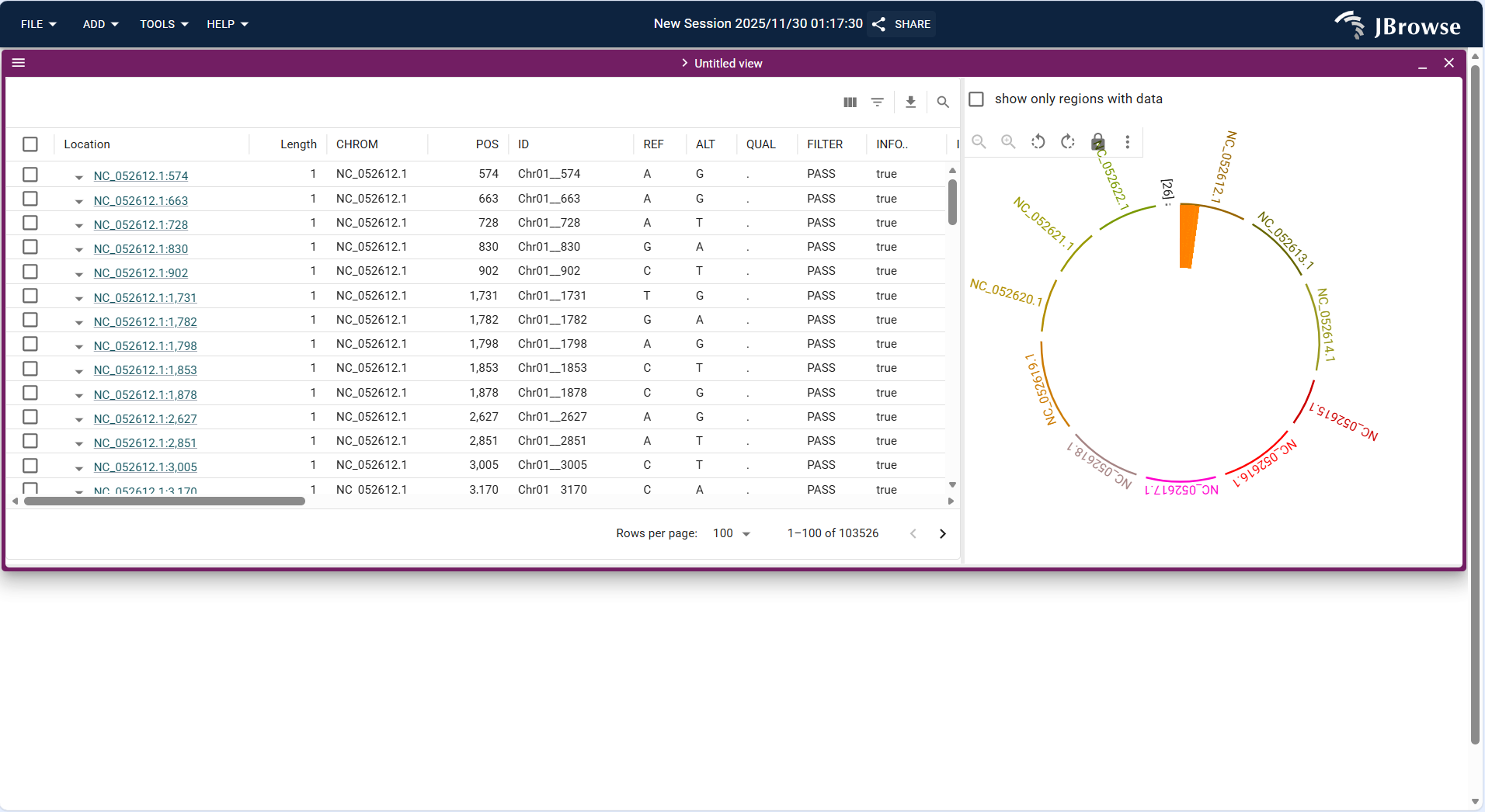
Figure 3.33: Screenshot of SV Inspector verifying Eucalyptus genome structural variation
3.3 Result Analysis
3.3.1 Single Track Result Analysis
3.3.1.1 Linear Genome View + Different Type Track Results
Overall Display Format
Centered on "linear coordinate axis + base sequence", the top shows the chromosome name and coordinate range (e.g., NC_052612.1:92,780,830..92,780,854), and the bases (A/T/C/G) are arranged in order below. Some versions support synchronous display of corresponding amino acid sequences (if it is a coding region).
Core Display Information
- Coordinate positioning: Precisely marks the genomic coordinates of the current view, supporting mouse drag or coordinate input for jumping to quickly lock the target region.
- Base distinction: Identifies 4 types of bases by different colors (default rules: A = green, T = red, C = blue, G = orange; adjustable in Preferences) for intuitive base type differentiation.
- Sequence integrity: Fully displays the original base sequence of the selected interval without missing or truncation (provided the FASTA file and index are complete).
- Zoom adaptation: Displays sequence abbreviations (e.g., only "ATCG..." placeholders) when the view is zoomed out, and clearly shows the specific type of each base when zoomed to the single-base level.
Interpretation Key Points
- Serves as the "basic positioning carrier" for all tracks; subsequent overlaid annotation, variation, and other tracks are in one-to-one correspondence with the coordinates of this sequence.
- Used to verify sequence accuracy (e.g., whether mismatched sites in alignment results are consistent with the reference sequence) and check the base composition of specific regions (e.g., TATA box sequence in the promoter region).
- For coding regions, combined with amino acid sequences, it can quickly determine whether variations cause amino acid changes (e.g., whether base G→A corresponds to amino acid Val→Ile).
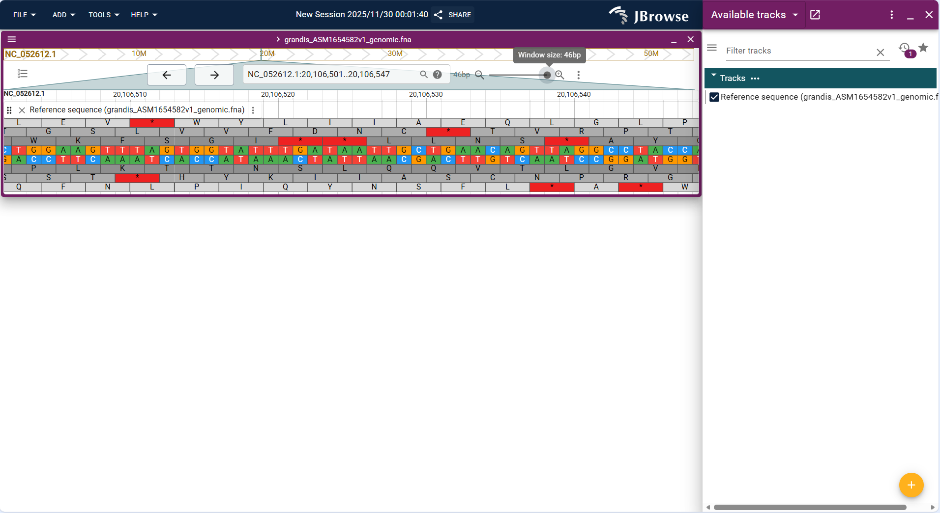
Figure 3.34: Screenshot of Linear Genome View with Reference Sequence Track
Overall Display Format
Above or below the reference sequence track, functional elements are displayed in the form of "rectangular blocks + connecting lines". Different types of elements are distinguished by different colors, and details can be viewed by hovering the mouse.
Core Display Information
- Element type and structure:
- Genes: Represented by complete rectangular blocks, with intron regions connected by thin lines and exons by thick rectangular blocks (intuitively distinguishing gene structure).
- Non-coding RNAs, regulatory regions: Represented by short rectangular blocks or line segments, labeled with corresponding type tags (e.g., "lncRNA", "enhancer").
- Attribute annotation: By default, displays gene ID or gene name; complete attributes (e.g., functional description, number of transcripts, chromosome location) can be viewed by hovering the mouse.
- Direction identification: Marks the transcription direction (5’→3’) of the gene with an arrow to clarify the expression strand of the gene.
- Hierarchical overlay: When multiple functional elements overlap (e.g., a gene overlaps with a repetitive sequence region), the hierarchy is automatically adjusted to avoid occlusion, and single elements can be viewed by clicking to expand.
Interpretation Key Points
- Quickly identify the distribution of functional elements in the target region (e.g., how many protein-coding genes are contained in a certain interval, and whether there are regulatory regions).
- Analyze gene structure characteristics (e.g., number of exons, intron length, whether there are alternatively spliced transcripts).
- Determine the functional association of variant sites (e.g., whether the variation is located in an exon, intron, or regulatory region, directly affecting the functional annotation of the variation).
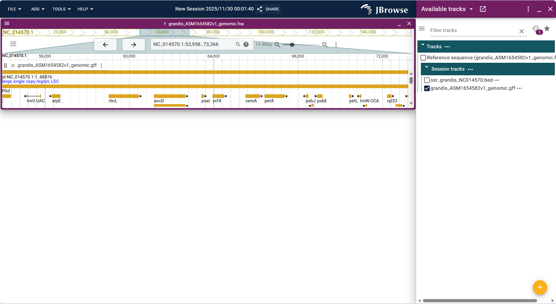
Figure 3.35: Screenshot of Linear Genome View with Feature Sequence Track
Overall Display Format
Centered on "custom interval highlight blocks", the track displays user-defined genomic regions (imported via BED files) as solid rectangular blocks above or below the reference sequence track. The blocks are colored uniformly by default (e.g., light blue) and can be customized in track settings for distinction.
Core Display Information
- Interval positioning: Each highlight block corresponds exactly to the "chromosome + start-end coordinates" in the BED file, with clear alignment to the genomic coordinate axis of the Linear Genome View.
- Label annotation: Supports displaying custom labels (e.g., "regulatory_region_1", "repeat_sequence_cluster") for each interval (configured via BED file's 4th column), which are displayed above the highlight blocks for quick identification.
- Batch display: Multiple non-overlapping intervals are arranged in sequence according to genomic coordinates; overlapping intervals are displayed in layers (without occlusion) or merged (configurable via track settings).
- Interactive operation: Clicking a highlight block pops up detailed information (e.g., exact coordinates, custom attributes in the BED file) for further verification.
Interpretation Key Points
- Visualize custom functional regions: Intuitively display the distribution of user-defined regions (e.g., regulatory elements, repetitive sequences, candidate target regions) on the genome.
- Correlate with other tracks: Overlay with Feature Track to analyze whether custom intervals overlap with genes/exons; overlay with Variant Track to check if variations are enriched in custom functional regions.
- Validate region accuracy: Verify whether the coordinates of predicted regions (e.g., computationally identified enhancer regions) match known functional elements.

Figure 3.36: Screenshot of Linear Genome View with Basic Track (custom regulatory region intervals in BED format)
Overall Display Format
Centered on "sequencing read alignment lines", the track displays each sequencing read (from BAM files) as a short horizontal line aligned to the reference sequence track. Reads are colored to indicate strand direction (e.g., forward strand = black, reverse strand = gray) and mismatches (e.g., red for A/C mismatch, blue for G/T mismatch) for intuitive differentiation.
Core Display Information
- Read alignment status:
- Mapped reads: Displayed as continuous lines aligned to the reference sequence, with mismatched bases marked by colored dots.
- Unmapped reads: Displayed as gray lines outside the reference sequence alignment range (or hidden by default, configurable via filter settings).
- Spliced reads: Intron regions are represented by broken lines (for RNA-seq data), reflecting the splicing pattern of transcripts.
- Quality indicators:
- Mapping quality (MAPQ): Reads with high MAPQ (e.g., ≥30) are displayed in bold; low-quality reads are displayed in light color or filtered out (adjustable via quality threshold settings).
- Base quality: Hovering over a base in a read displays its Phred quality score (e.g., Q30 = 99.9% accuracy) for evaluating data reliability.
- Coverage depth: A coverage histogram is displayed at the top of the track, with the vertical axis representing the number of reads covering each position (depth) and the horizontal axis corresponding to genomic coordinates.
Interpretation Key Points
- Evaluate alignment quality: Check the uniformity of read coverage (avoiding extreme high/low coverage regions) and the proportion of mismatched bases (indicating potential sequencing errors or true variations).
- Verify variation authenticity: For variant sites in the Variant Track, check if the aligned reads support the variation (e.g., whether most reads at the site carry the alternative allele).
- Analyze splicing patterns: For RNA-seq data, identify alternative splicing events (e.g., exon skipping, intron retention) via spliced read breakpoints.
- Detect structural variations: Abnormal alignment patterns (e.g., read pairs mapped to distant regions, split reads) indicate potential deletions, duplications, or translocations.
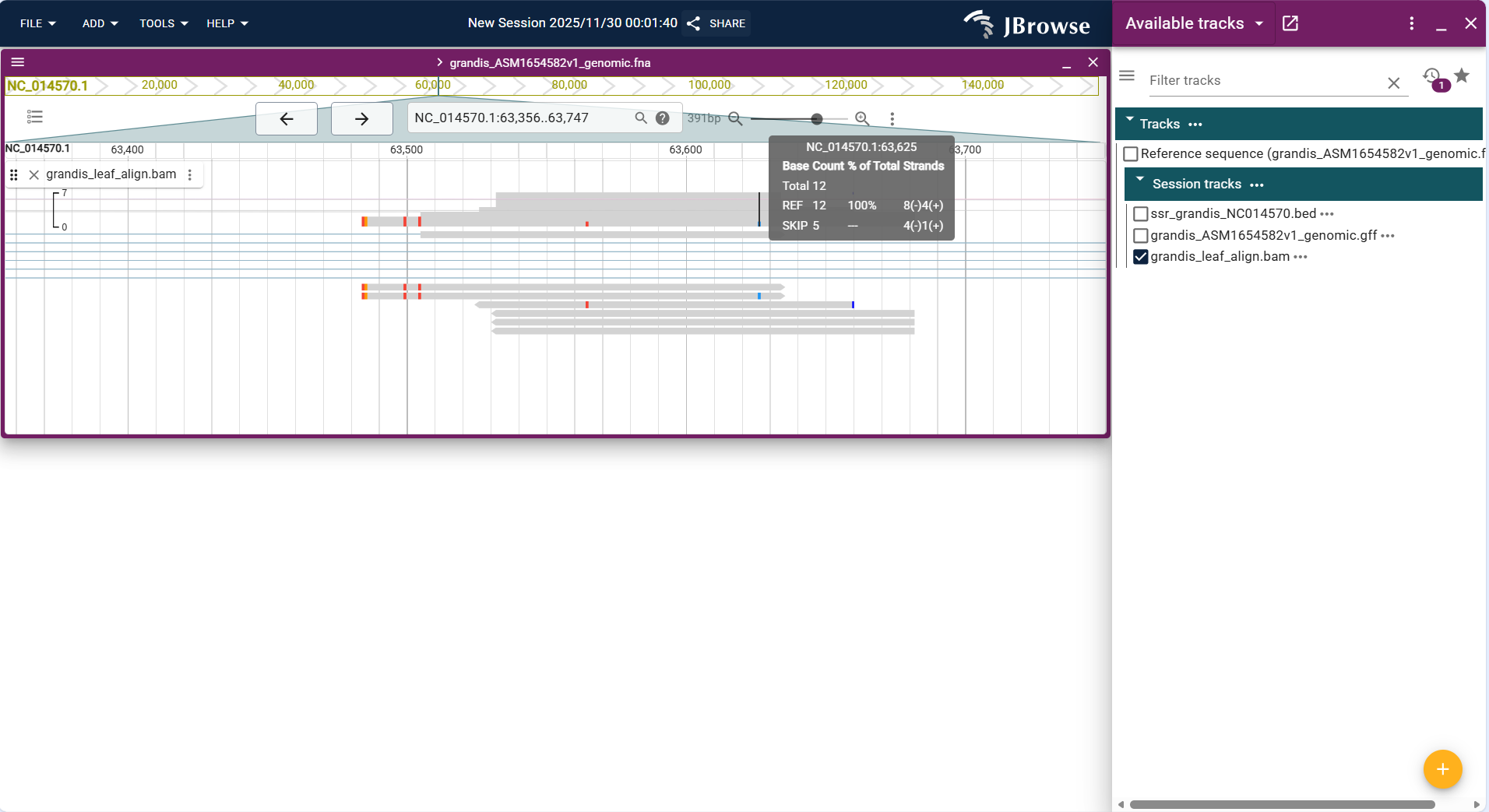
Figure 3.37: Screenshot of Linear Genome View with Alignments Track (RNA-seq read alignment data in BAM format)
Overall Display Format
In the Linear Genome View, single nucleotide variation (SNV) sites are displayed in the form of "coordinate labels + variation type annotations". Each variant site directly marks the genomic coordinate (e.g., S6_28828705) and variation type (e.g., SNV C->T), arranged in the order of genomic coordinates. When there is no distinction by shape/color, they are displayed as clear blue text labels by default, and details of the variation can be viewed by clicking.
Core Display Information
- Variation coordinate and type:
- Each marker clearly indicates the genomic coordinate and single nucleotide variation type.
- Precise position correspondence:
- The position of the variation label is completely consistent with the genomic coordinate, intuitively presenting the exact position of each SNV on the genome.
- Batch distribution presentation:
- Multiple SNVs are arranged in coordinate order, and each variation is clearly displayed when there is no overlap, facilitating observation of the distribution density of variations.
Interpretation Key Points
- Variation distribution and density analysis:
- Quickly identify the number and distribution pattern of SNVs in the target region (e.g., how many SNVs are in a certain interval, and whether there is an aggregation phenomenon).
- Variation type preference:
- Analyze the base substitution preference of SNVs in this region (e.g., substitutions such as C->T and A->G are predominant in the screenshot, which can infer whether there is a preference for base editing or mutation mechanisms).
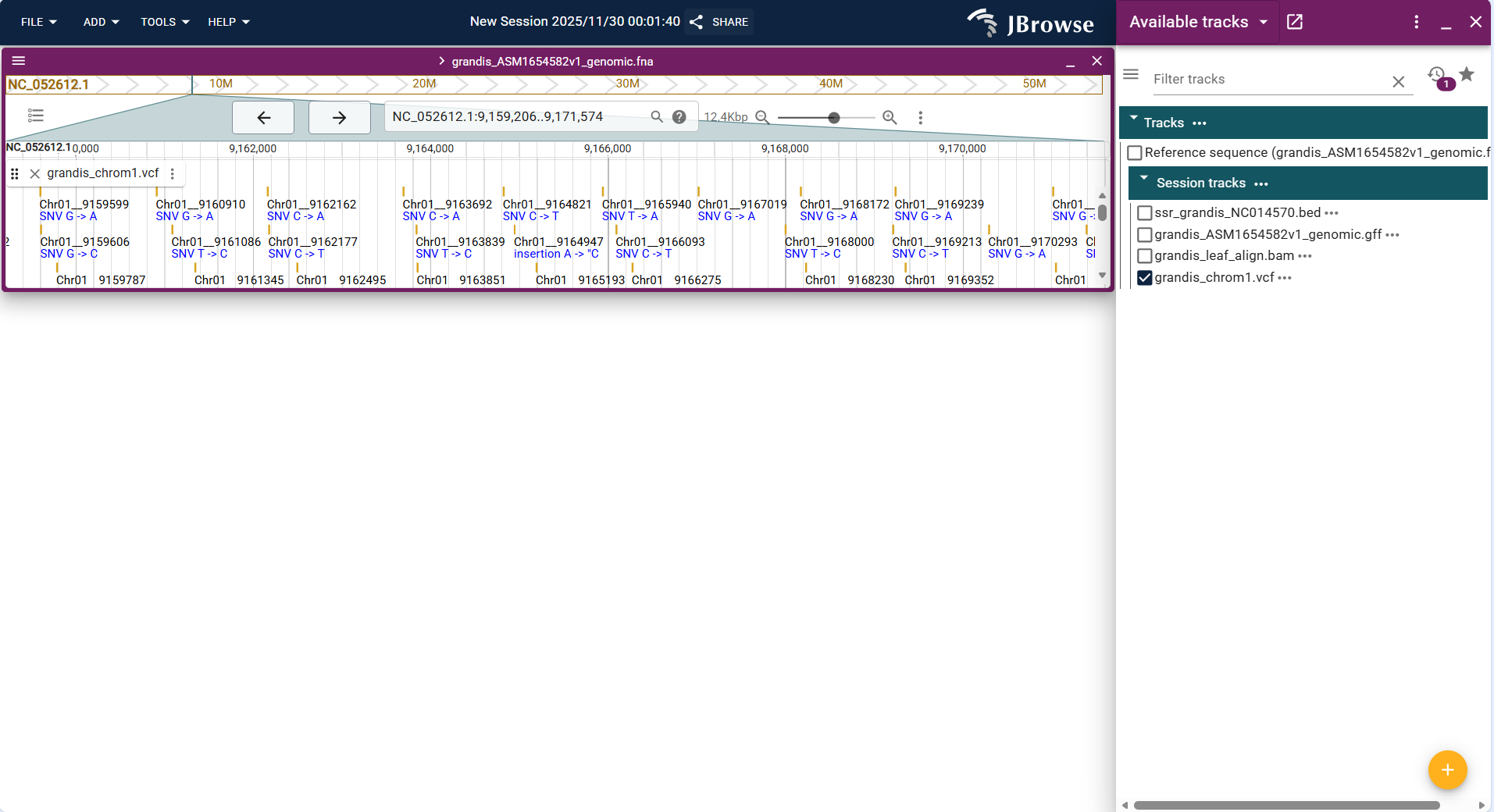
Figure 3.38: Screenshot of Linear Genome View with Variant Track
Overall Display Format
Centered on "line chart", the vertical axis represents quantitative values (e.g., alignment signal intensity in this track), the horizontal axis corresponds to genomic coordinates (NC_014570.1:100,278..112,392), and the height of the blue line reflects the magnitude of the quantitative value.
Core Display Information
- Value trend: Displays the genomic distribution of alignment signal intensity through continuous blue lines (e.g., local signal peaks correspond to regions with high alignment density).
- Value annotation: When hovering the mouse over the line (especially peak positions), the exact quantitative value (e.g., signal intensity) will be displayed.
- Single-track distinction: The track uses a unified blue line to present the data, with the vertical axis range (0~20000) matching the value scale of this dataset.
- Coordinate matching: The horizontal axis is strictly aligned with the genomic coordinate system, ensuring the data corresponds to the correct genome region.
Interpretation Key Points
- Identify high-signal regions of the dataset (e.g., the prominent blue peak in the figure corresponds to a region with concentrated alignment signals, which may be a functionally active genomic region).
- Analyze the association between the quantitative signal and genomic structure (e.g., whether the signal peak is located in a gene region or regulatory region).
- Evaluate data distribution characteristics (e.g., the sparse signal in most regions indicates low alignment density in those genomic segments).
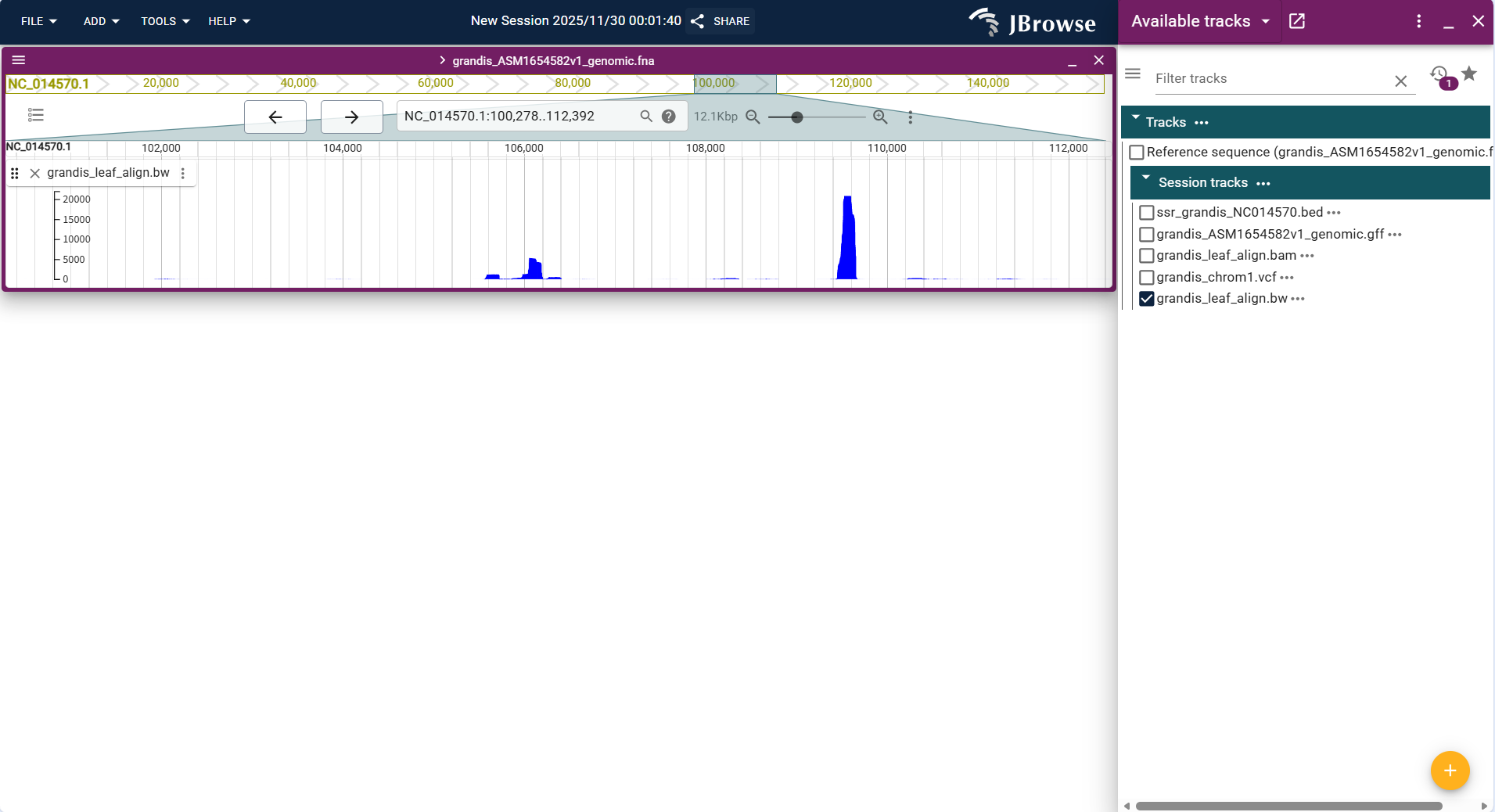
Figure 3.39: Screenshot of Linear Genome View with Quantitative Track
Overall Display Format
Centered on "parallel line charts for multiple datasets", the vertical axis of each sub-track represents the quantitative value of the corresponding dataset (e.g., alignment signal intensity of different samples), the horizontal axis shares the same genomic coordinates (NC_052617.1:28,436,577..28,796,772), and the height of lines in each sub-track reflects the value magnitude of the respective dataset.
Core Display Information
- Multi-group value trend: Displays the genomic distribution of quantitative data for two datasets (grandis_leaf_align.bw and grandis_Symbiotic_tissue_align.bw) through parallel lines, enabling direct visual comparison of trends.
- Dataset distinction: Each dataset corresponds to an independent sub-track, with clear labels (dataset file names) to distinguish between different samples/groups.
- Value annotation: Hovering the mouse over the line in any sub-track will display the exact quantitative value of that dataset at the corresponding position.
- Coordinate consistency: The shared horizontal axis ensures that the quantitative data of different datasets are aligned to the same genomic region for comparative analysis.
Interpretation Key Points
- Compare the signal distribution differences between multiple datasets (e.g., the signal peaks of the two samples in the figure have different positions and intensities, indicating differences in alignment density between the leaf and symbiotic tissue samples).
- Identify common high-signal regions (e.g., the overlapping weak signal segments in both sub-tracks correspond to genomic regions with low alignment density in both samples).
- Analyze sample-specific characteristic regions (e.g., the unique prominent peak in one sub-track corresponds to a genomic region with sample-specific high alignment signals).
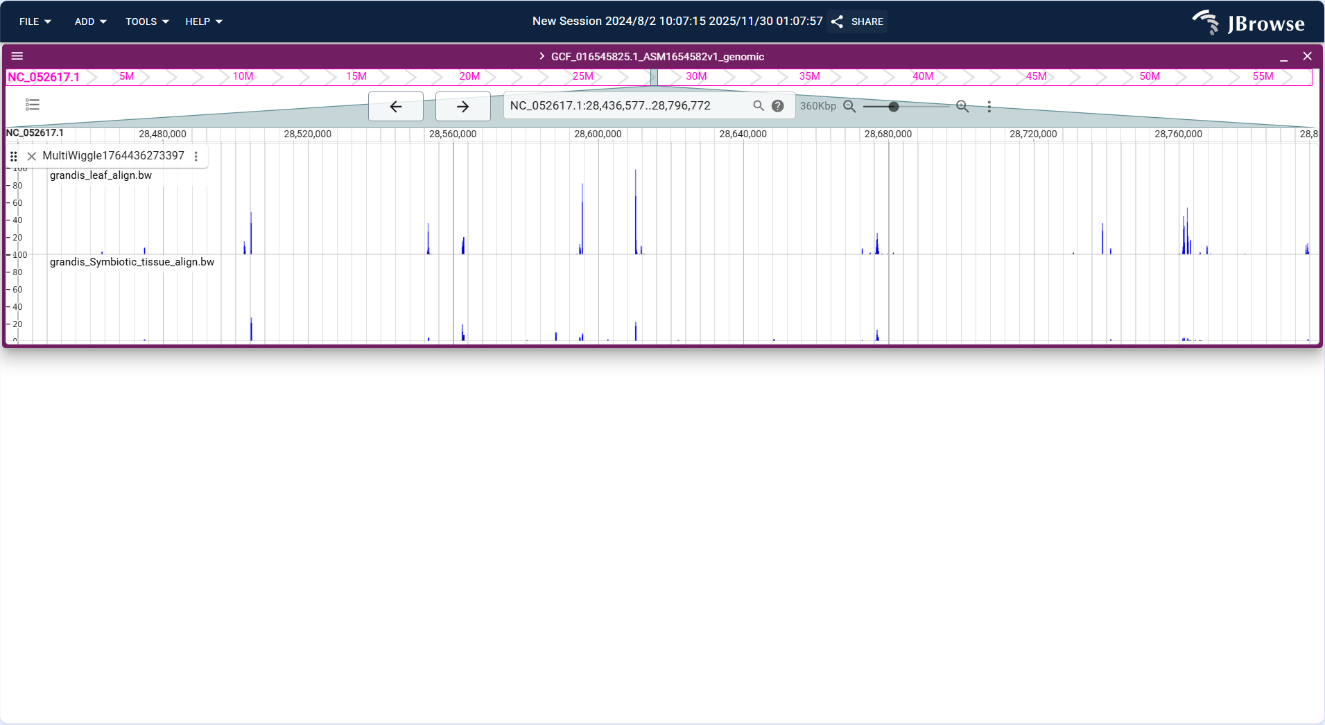
Figure 3.40: Screenshot of Linear Genome View with Multi-quantitative Track
Overall Display Format
Centered on "sliding window line chart", the horizontal axis represents genomic coordinates, and the vertical axis represents GC content percentage (0%-100%). The track calculates GC content (proportion of G+C bases) for each sliding window (default 100bp, configurable) based on the reference sequence and displays it as a continuous line.
Core Display Information
- Window size adaptation: Supports adjusting the sliding window size; smaller windows show local GC content fluctuations, while larger windows display overall distribution patterns.
- Baseline reference: A horizontal baseline at 50% GC content is displayed by default to quickly distinguish GC-rich (above baseline) and AT-rich (below baseline) regions.
- Value annotation: Hovering the mouse over any position on the line displays the exact GC content value and window coordinates.
- Region highlighting: Supports manual selection of a genomic interval to calculate and display the average GC content of the interval.
Interpretation Key Points
- Identify functional region characteristics: GC-rich regions are often associated with gene-dense regions (e.g., exons, CpG islands), while AT-rich regions may correspond to intergenic regions or repetitive sequences.
- Validate genome assembly quality: Abnormal GC content fluctuations (e.g., sudden spikes/drops) may indicate assembly errors or contamination (e.g., bacterial sequence insertion).
- Correlate with other tracks: Overlay with Feature Track to check if gene exons have higher GC content than introns; overlay with Quantitative Track to analyze whether GC-rich regions are associated with high gene expression.
- Support comparative genomics: Compare GC content distribution of homologous regions between different species to infer evolutionary conservation.
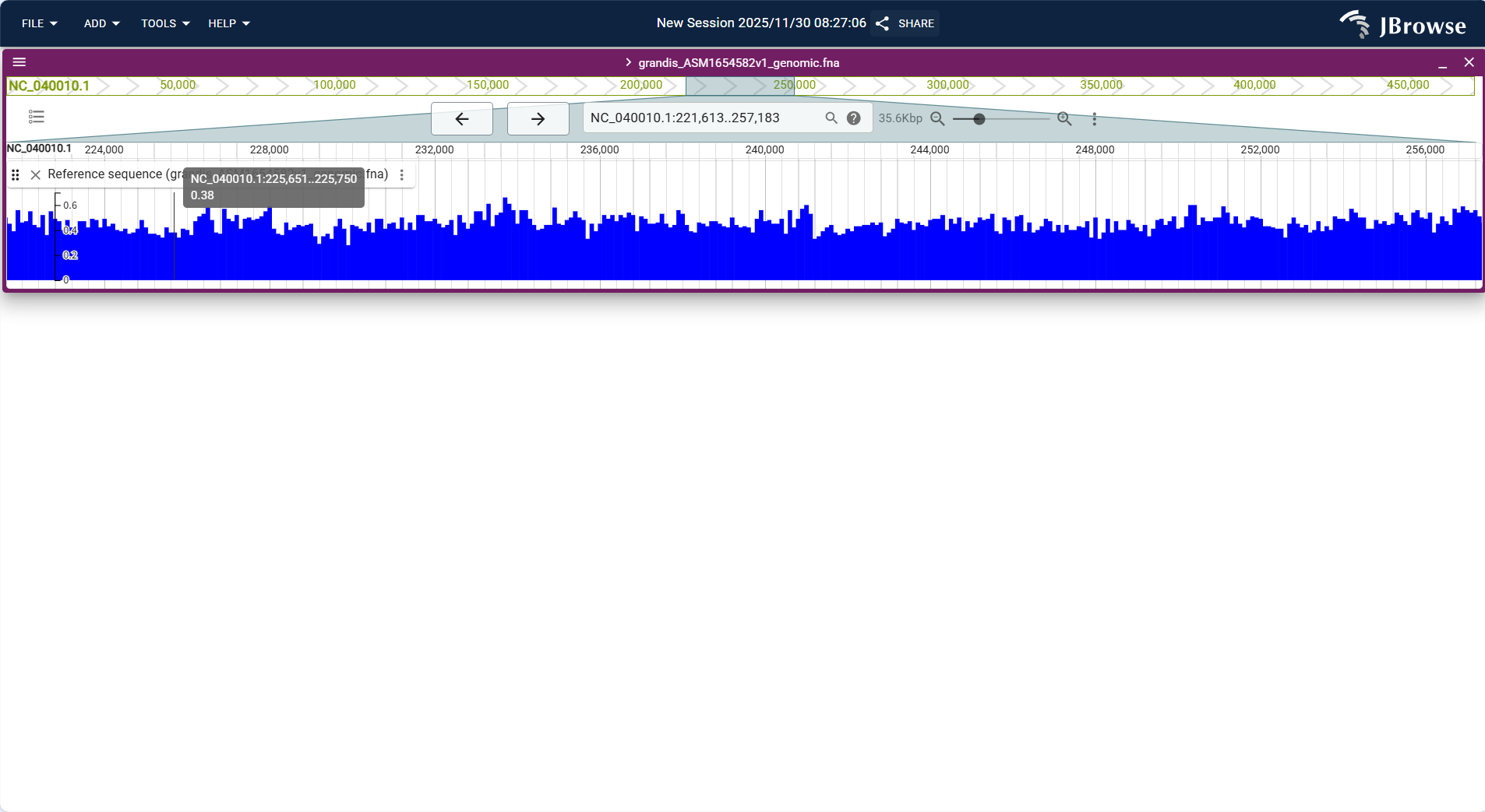
Figure 3.41: Screenshot of Linear Genome View with GC Content Track
Overall Display Format
Centered on "synteny blocks + homology connection lines", the horizontal axis corresponds to the coordinate range (17,259,500..33,335,673) of the target genome (NC_052612.1). Blocks of different colors represent homologous sequence fragments with another genome, and the connection lines between blocks correspond to the positional linkage of homologous fragments in the two genomes.
Core Display Information
- Synteny block identification: Blocks in colors (e.g., red, purple) represent homologous sequence fragments between the two genomes, and the length of each block corresponds to the genomic span of the fragment.
- Homology relationship linkage: The connection lines between blocks (e.g., the short lines corresponding to red blocks) intuitively reflect the positional correspondence of homologous fragments in the two genomes.
- Coordinate matching: The horizontal axis is strictly aligned with the coordinate system of the target genome, ensuring one-to-one correspondence between syntenic regions and specific genomic positions.
- Fragment continuity: The continuous distribution of blocks reflects the synteny level of the two genomes in this region (dense blocks correspond to regions with high synteny).
Interpretation Key Points
- Identify synteny-enriched regions: The continuously distributed red blocks in the figure correspond to segments with high synteny between the two genomes, reflecting strong sequence conservation in these regions.
- Analyze sequence variation regions: Gaps with interrupted blocks or no continuous blocks may be locations where genomic rearrangement, insertion/deletion, or other variation events occur.
- Locate homologous fragments: Through blocks and connection lines, the specific coordinates of homologous sequences in the two genomes can be quickly matched, providing positional basis for subsequent functional homology analysis.
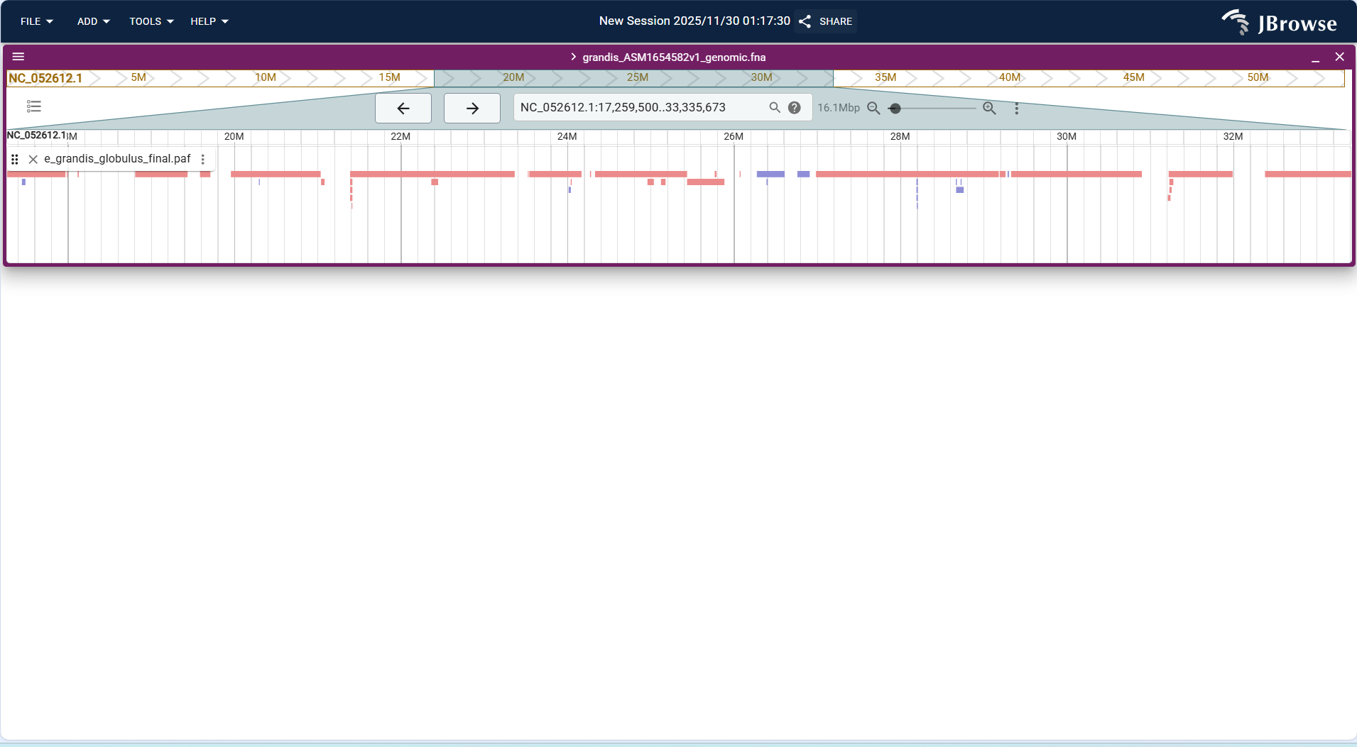
Figure 3.42: Screenshot of Linear Genome View with Synteny Track
Overall Display Format
Centered on a "square heatmap", both the horizontal and vertical axes are genomic coordinates. The depth of the heatmap color indicates the chromatin interaction intensity, supporting adjustment of resolution and thresholds to focus on key interaction regions.
Core Display Information
- Interaction intensity: Default rule (darker color indicates stronger interaction; e.g., yellow = weak interaction, red = strong interaction), intuitively distinguishing interaction differences in different regions.
- Resolution adaptation: Supports switching resolutions (e.g., 10kb, 50kb, 100kb); low resolution shows global interaction patterns, and high resolution views fine interactions (e.g., chromatin loops).
- Structural features:
- Topologically Associating Domains (TADs): Represented by "square-shaped" heatmap blocks with strong internal interactions and weak external interactions, which are the basic units of genomic 3D structure.
- Chromatin loops: Represented by "spot-like" high-value regions in the heatmap, indicating direct interactions between two distal regions (e.g., promoter-enhancer interactions).
- Coordinate correspondence: The horizontal/vertical axis coordinates of the heatmap are completely consistent with the reference sequence and Feature tracks, facilitating the association of 3D structure with one-dimensional functional elements.
Interpretation Key Points
- Identify genomic 3D structure features (e.g., TAD boundary positions, number and distribution of chromatin loops).
- Analyze the 3D association of functional elements (e.g., whether enhancers form interactions with target genes through chromatin loops to regulate gene expression).
- Compare Hi-C heatmaps of different samples (e.g., normal tissue vs tumor tissue) to discover disease-related 3D structure abnormalities (e.g., disappearance of TAD boundaries, formation of new chromatin loops).
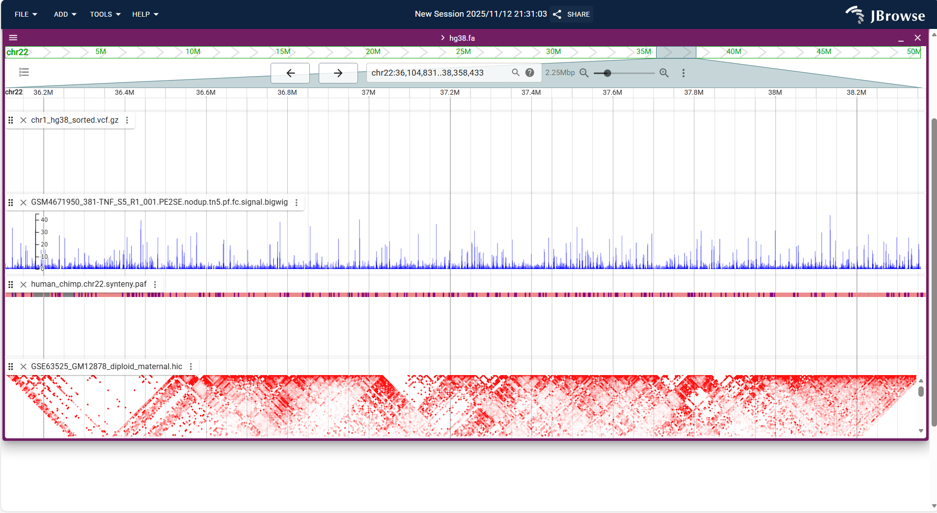
Figure 3.43: Screenshot of Linear Genome View with Hi-C Track
3.3.1.2 Circular View + Different Type Track Results
Overall Display Format
Centered on the target genome (grandis_ASM165458v2L_genomic.fna), a circular genome layout is constructed. Arcs of different colors correspond to distinct sequence segments of the genome (e.g., sequences labeled NC_052621.1, NC_052612.1, etc.), while local highlighted markers (such as the orange short block) are used to showcase specific regions/features. All sequence segments are arranged continuously along the circle according to genomic coordinates, presenting a circular visualization structure of the entire genome.
Core Display Information
- Precise positioning: Each arc corresponds to a specific genomic sequence (distinguished by identifiers like NC_0526xx.1), and its position on the circle matches the genomic coordinates of the corresponding sequence. Highlighted markers (e.g., the orange block) are anchored to designated regions of the target sequence.
- Region details: Hovering the mouse over an arc or highlighted marker will pop up detailed annotation information, such as the sequence ID, coordinate range, and feature type.
- Batch distribution: Arcs of different colors distinguish different genomic sequence segments, which are arranged continuously along the circle to fully present the fragmented structural layout of the entire genome.
- View function: Supports zoomed-in viewing of specific sequence segments/markers, and allows focusing on target regions via filtering functions (e.g., filtering by sequence ID).
Interpretation Key Points
- Analyze genome structure: Visually observe the relative positions and distribution ranges of each sequence segment in the whole genome through the circular layout, and clarify the arrangement relationships of different segments.
- Locate target regions: Quickly pinpoint key focus regions in the genome (e.g., segments containing functional genes or characteristic elements) using highlighted markers (such as the orange block).
- Link annotation information: Associate the NC_0526xx.1 sequence IDs corresponding to the arcs with the genome’s annotation database to obtain attributes like the function and annotation type of each segment.
- Compare genomic differences: Later, overlay the circular views of other samples (e.g., different Eucalyptus ecotypes) to compare the layout and feature differences of corresponding sequence segments, and identify sample-specific genomic structures.

Figure 3.44: Screenshot of Circular View with Variant Track
3.3.1.3 Dotplot View + Single Type Track Result
Overall Display Format
Centered on a "two-dimensional scatter plot", the horizontal axis (x-axis) represents the reference genome (e.g., Eucalyptus grandis chr1) and the vertical axis (y-axis) represents the query genome (e.g., Myrtus communis chr1). Each dot in the plot represents a homologous segment between the two genomes, with the dot's position corresponding to the coordinates of the segment in the reference and query genomes.
Core Display Information
- Coordinate scaling: Both axes use linear genomic coordinates, with consistent scaling to ensure proportional display of segment lengths. Axis labels indicate chromosome names and coordinate ranges.
- Homology direction:
- Forward homology (sequence direction consistent): Dots are distributed near the main diagonal (y=x) of the plot, forming diagonal dot clusters.
- Reverse homology (sequence direction reversed, inversion event): Dots are distributed near the anti-diagonal (y=-x + C), forming reverse diagonal dot clusters.
- Similarity coding: Dot color depth reflects sequence similarity of homologous segments (darker dots = higher similarity, lighter dots = lower similarity), based on similarity scores in the PAF file.
- Interactive query: Hovering over a dot displays detailed information (e.g., reference segment coordinates, query segment coordinates, similarity percentage, alignment length).
Interpretation Key Points
- Evaluate overall collinearity: Dots concentrated near the main diagonal indicate high collinearity between the two genomes (few rearrangement events); scattered dots indicate low collinearity.
- Identify rearrangement events:
- Inversion: Reverse diagonal dot clusters (off the main diagonal) indicate chromosome inversion in the query genome relative to the reference.
- Translocation: Dot clusters far from the main diagonal indicate inter-chromosomal translocation.
- Duplication: Multiple dots in the y-axis direction corresponding to a single x-axis position indicate segment duplication in the query genome.
- Localize conserved segments: Dense dot clusters near the main diagonal represent highly conserved homologous segments (e.g., functional gene clusters) between the two genomes.
- Validate genome assembly: Abnormal dot distribution (e.g., fragmented dots) may indicate assembly errors in the reference or query genome (e.g., misassembled contigs).

Figure 3.45: Screenshot of Dotplot View with Synteny Track
3.3.1.4 Linear Synteny View + Single Type Track Result
Overall Display Format
Centered on "dual-genome parallel tracks + global homology connection lines", the upper track corresponds to the genome globus_ASM4622685v1_genomic.fna and the lower track corresponds to grandis_ASM1654582v1_genomic.fna; the horizontal axes display the sequence coordinates of the two genomes respectively, and the dense red lines in the middle represent the correspondence of homologous sequence fragments between the two genomes.
Core Display Information
- Dual-genome layout: The two target genomes are displayed in separate upper/lower tracks, clearly distinguishing the two sequences to be compared.
- Homology connection lines: Dense red lines intuitively link homologous fragments between the two genomes, reflecting the positional correspondence of conserved sequences.
- Genome coordinates: The upper track shows the coordinate range of the globus genome, while the lower track matches the coordinate system of the grandis genome, ensuring positional alignment of homologous regions.
- Track status: Both genome tracks display "No tracks active" (specific data tracks can be enabled via the "OPEN TRACK SELECTOR" button to show detailed sequence/feature information).
Interpretation Key Points
- Track status: Both genome tracks display "No tracks active" (specific data tracks can be enabled via the "OPEN TRACK SELECTOR" button to show detailed sequence/feature information).
- Complex rearrangement regions: The crisscrossing of red lines suggests potential genomic rearrangement events (e.g., inversions, translocations) in the corresponding segments.
- Follow-up analysis tips: Activating specific tracks (via "OPEN TRACK SELECTOR") allows viewing detailed sequence or functional feature information, which helps refine the analysis of homologous fragment functions and evolutionary relationships.

Figure 3.46: Screenshot of Linear Synteny View with Synteny Track
3.3.1.5 Spreadsheet View + Different Type Track Results
Overall Display Format
Centered on a "tabular data table", the view displays functional elements (imported via GFF3/GTF files) as rows and their attributes as columns. The table supports sorting, filtering, and searching functions for batch management of functional elements.
Core Display Information
- Standard attribute columns:
- Basic information: Chromosome (Chr), start coordinate (Start), end coordinate (End), strand direction (Strand, +/-, . for unknown).
- Element type: Feature Type (e.g., gene, exon, mRNA, lncRNA).
- Annotation information: ID (unique identifier), Name (gene name/alias), Description (functional description), Source (annotation source, e.g., Gencode).
- Additional attributes: Transcript ID (for exons), Parent (parent element ID, e.g., exon's parent mRNA ID) – derived from GFF3/GTF file attributes.
- Interactive operations:
- Sorting: Click column headers to sort by ascending/descending order (e.g., sort by Start coordinate to arrange elements by genomic position).
- Filtering: Use column filters to screen elements (e.g., filter Feature Type = "gene" to display only genes, filter Strand = "+" to display forward-strand elements).
- Searching: Global search box to find elements by ID, Name, or coordinate.
- Linkage to Linear View: Clicking a row jumps to the corresponding element's position in the Linear Genome View for visualization verification.
Interpretation Key Points
- Batch management of functional elements: Efficiently browse, sort, and filter large-scale annotation data (e.g., thousands of genes) without visual occlusion from the Linear View.
- Screen target elements: Filter elements by specific conditions (e.g., genes located on chr1, exons of mRNA transcripts) for subsequent analysis (e.g., differential expression gene annotation).
- Verify annotation consistency: Check for duplicate IDs, conflicting coordinates, or missing attributes (e.g., exons without Parent IDs) to ensure annotation file quality.
- Export for downstream analysis: Support exporting filtered/sorted tables as CSV/TSV files for further analysis in software such as Excel, R, or Python.

Figure 3.47: Screenshot of Spreadsheet View with Feature Track
Overall Display Format
Centered on a "variant attribute table", the view displays variation sites (imported via VCF/VCF.gz files) as rows and their genetic/quality attributes as columns. The table supports advanced filtering and batch processing for efficient variation data management.
Core Display Information
- Standard attribute columns:
- Position information: Chromosome (Chr), position (Pos), reference allele (REF), alternative allele (ALT).
- Quality control: QUAL (variation quality score), FILTER (filter status, e.g., PASS, LowQual), DP (read depth), MQ (mapping quality).
- Genetic attributes: Variant Type (SNV, Indel, MNPs), AF (allele frequency), AC (allele count), AN (total allele number).
- Functional annotation: Ann (functional impact, e.g., synonymous_variant, missense_variant), Gene (affected gene), Feature (affected functional element, e.g., exon).
- Advanced operations:
- Multi-condition filtering: Combine column filters (e.g., FILTER = "PASS", QUAL > 50, Variant Type = "SNV") to screen high-confidence variations.
- Custom columns: Select to display/hide attributes (e.g., hide low-value columns like FORMAT to simplify the table).
- Linkage to Linear View: Click a row to jump to the variation's position in the Linear Genome View, overlaying with Alignments Track for verification.
- Batch export: Export filtered variations as CSV/VCF files for downstream analysis (e.g., association mapping, haplotype analysis).
Interpretation Key Points
- Quality control of variation data: Filter out low-quality variations (e.g., QUAL < 30, FILTER ≠ "PASS") to ensure reliability of subsequent analysis.
- Functional prioritization of variations: Screen variations with functional impacts (e.g., missense_variant, stop_gained) in candidate genes for experimental verification.
- Statistical analysis of variation characteristics: Count variation types (SNV vs Indel ratio), allele frequencies (common vs rare variations), and chromosome distribution.
- Data integration: Combine with Feature Track spreadsheets to cross-verify whether high-confidence variations are located in functional gene regions.

Figure 3.48: Screenshot of Spreadsheet View with Variant Track
3.3.1.6 SV Inspector + Single Type Track Result
Overall Display Format
Centered on "variant detail table + circular genome visualization", the left panel displays a tabular list of variant sites with their attribute information, while the right panel presents the genome as a circular structure; the two panels are linked to show the correspondence between variant details and their genomic positions.
Core Display Information
- Variant table (left): Contains columns such as Location (variant genomic position, e.g., NC_052612.1:574), Length (variant length, here all 1bp, indicating single nucleotide variants), CHROM (chromosome), POS (site coordinate), REF (reference base), ALT (variant base), QUAL (quality value), FILTER (filter status, marked "PASS" here), and INFO (additional annotations). The table supports pagination (showing 1-100 of 103526 variants) and row expansion.
- Circular genome view (right): Arranges genome sequences (e.g., NC_052612.1, NC_052613.1) in a circular layout; the orange block marks the genomic region corresponding to the variants listed in the table, intuitively showing the variant’s position on the genome.
- Linkage function: Selecting a variant in the table will synchronously locate its position in the circular view, and vice versa.
Interpretation Key Points
- Batch browse variant details: The table allows quick screening and viewing of the attribute information of a large number of variants (e.g., distinguishing transition/transversion types via REF/ALT columns).
- Intuitive genomic positioning: The circular view quickly shows the distribution of variants on the genome (e.g., the orange block indicates a variant-enriched region), avoiding the limitation of linear view for global genomic positioning.
- Cross-validation of variant information: Combine the table’s detailed attributes (e.g., "PASS" filter status) with the circular view’s positional information to analyze whether variants are concentrated in specific functional regions (e.g., gene coding regions).

Figure 3.49: Screenshot of SV Inspector with Variant Track